Quality Control and
Data Processing

HC PLOTS
Bad pixels and Ratio, RON, GAIN, linearity
QC1 database (advanced users): browse | plot

Detector frames are used to measure the basic characteristics of the detectors which are needed to calibrate the data.
They are also used to monitor the health and technical performance of the two detectors (HAWAII-2RG: MATISSE-LM and AQUARIUS: MATISSE-N.
These detector calibrations cover the static flatfield (FLATFIELD), the Bad Pixel Map (BADPIX) and the non-linearity map (NONLINEARITY)

They are recorded periodically or after a detector intervention in different read-out modes:

• HAWAII-R2G: FAST-SPEED and SLOW-SPEED
  
• AQUARIUS: HIGH-GAIN and LOW-GAIN
  

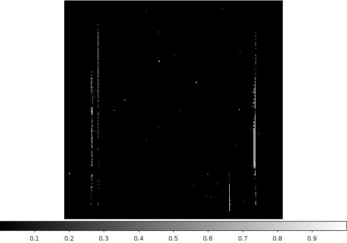
	Bad Pixel Map hawaii detector
	Bad Pixel Map aquarius detector

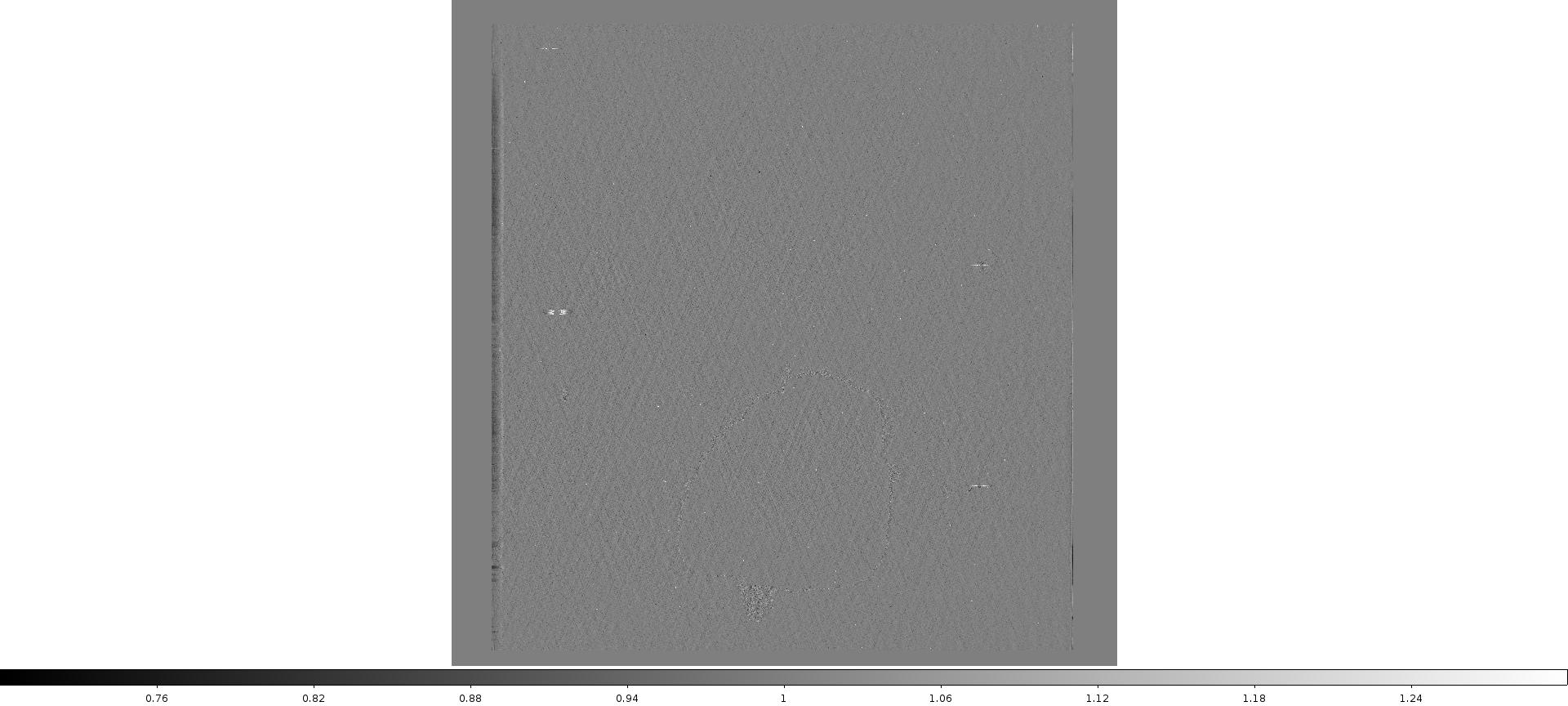	Flat field Map hawaii detector
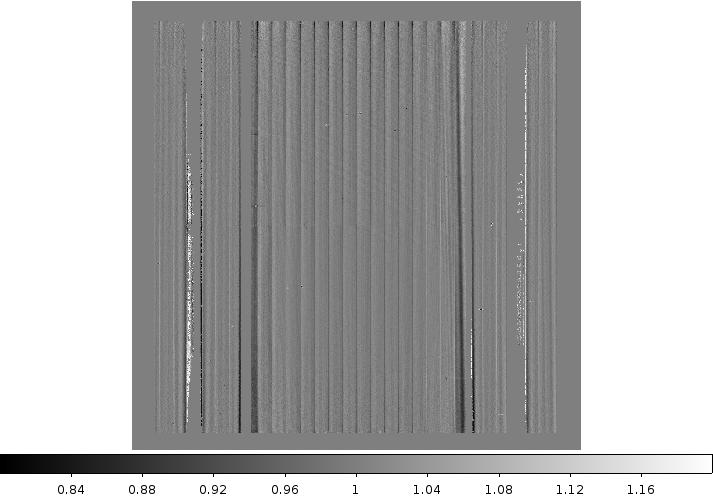	flat field Map aquarius detector

The product contains an image of the full detector (2048x2048 for the L/M detector and 1024x1024 for the N detector) where the badpixels are marked by 1 and the good pixels by 0.
A bad pixel on the detector which is set to unity (1) in the static mask gets excluded from the general bad pixel counts.
The number of bad pixels depends of the detector and the readmode.

QC1_parameters

FITS key	QC1 database: table, name	definition	class*	HC_plot**	more docu
QC.DET..BADPIX	matisse_detector..badpix	number of bad pixels	HC		[docuSys coming]
QC.DET..GOODPIX	matisse_detector..goodpix	number of good pixels			[docuSys coming]
QC.DET..GOODPIXELRATIO	matisse_detector..ratio_goodbad	ratio good over total pixels	HC		[docuSys coming]
*Class: KPI - instrument performance; HC - instrument health; CAL - calibration quality; ENG - engineering parameter **There might be more than one.

Trending

The QC parameters badpix and ratio_goodbad are trended for both detectors and the different readout modes. The number of BADPIX is shown in the trending plots.

Scoring&thresholds Bad Pixels

The different QC parameters are scored based on values provided by the consortium.

History

The evolution of the number of BADPIX will be shown under "FULL" once more data have been accumulated.

Algorithm Bad Pixels

The recipe used is mat_cal_det which also produces the FLATFIELD and the NONLINEARITY maps.
For each pixel, a temporal median and variance is calculated.
The raw statistics of the flatfield exposures contain the dark statistics (pixel offset and dark noise) which is subtracted from the flat field statistics of the same DIT.
From all dark statistics values of a pixel, an average median and variance is calculated and scaled to a detector dependent time scale. This dark median contains electronic effects (ramps) which are estimated and stored as dark median reference. The residuals are used to detect bad pixels for the preliminary bad pixel map.
From the compensated flat field statistics of each pixel, a mapping from raw to calibrated intensities is calculated. For the Aquarius detector, a global flux dependend nonlinearity law is estimated. For the HAWAII-2RG detector a intensity dependend nonlinearity mapping using a simple function is determined. Together with the nonlinearity mapping, a pixel (HAWAII-2RG) or detector (Aquarius) specific compensation limit is calculated.
The nonlinearity compensation is used to derive from all flat field statistics below the saturated intensity an average median and variance scaled to a detector specific time scale. These two values (median and variance) for each pixel represents the illumination intensity and photon noise (and EN for the Aquarius). This flat field median is influenced by the inhomogenoius illumination which is estimated and stored as flat field median reference. The factor between flat field median and flat field median reference is used as flat field value for each pixel. A test is used to set the flat field factor to 1.0 for pixels with low illumination.
The final bad pixel map is derived from the dark median reference and the flat field median reference.

The product contains in the primary HDU the flat field map for the given detector. The standard error map is stored in an extension.
The value of the flat field map is set to 1 if no valid flatfield can be calculated and the error is set to a very large value. This flat field map is different from the observation specific flatfield (pro.catg OBS_FLATFIELD)

QC1_parameters

The header of the FLATFIELD product contains QC parameters describing the full detector (see table below) as well as the detectro channels. The QC parameters for each detector channel will be used further to convert the pixel values from DU into electrons for the OBS_FLATFIELD.

FITS key	QC1 database: table, name	definition	class*	HC_plot**	more docu
QC.DET..RON	matisse_detector..ron_detflat	Flat Field Map detector noise (electron)	HC		[docuSys coming]
QC.DET..GAIN	matisse_detector..gain_detflat	Flat Field Map conversion factor (electron/DU)	HC		[docuSys coming]
QC.DET..FFM.STDEV	matisse_detector..stdev_nonlin	Non Linearity Map standard deviation	HC		[docuSys coming]
*Class: KPI - instrument performance; HC - instrument health; CAL - calibration quality; ENG - engineering parameter **There might be more than one.

Trending

The QC parameters RON and Gain are trended for both detectors and the different readout modes. They are shown in the trending plots.

Scoring&thresholds Flat Field Map

The different QC parameters are scored based on values provided by the consortium.

History

The evolution of the number of BADPIX will be shown under "FULL" once more data have been accumulated.

Algorithm Flat Field Map

The recipe used is mat_cal_det which also produces the BADPIX and the NONLINEARITY maps.
For each pixel, a temporal median and variance is calculated.
The raw statistics of the flatfield exposures contain the dark statistics (pixel offset and dark noise) which is subtracted from the flat field statistics of the same DIT.
From all dark statistics values of a pixel, an average median and variance is calculated and scaled to a detector dependent time scale. This dark median contains electronic effects (ramps) which are estimated and stored as dark median reference. The residuals are used to detect bad pixels for the preliminary bad pixel map.
From the compensated flat field statistics of each pixel, a mapping from raw to calibrated intensities is calculated. For the Aquarius detector, a global flux dependend nonlinearity law is estimated. For the HAWAII-2RG detector a intensity dependend nonlinearity mapping using a simple function is determined. Together with the nonlinearity mapping, a pixel (HAWAII-2RG) or detector (Aquarius) specific compensation limit is calculated.
The nonlinearity compensation is used to derive from all flat field statistics below the saturated intensity an average median and variance scaled to a detector specific time scale. These two values (median and variance) for each pixel represents the illumination intensity and photon noise (and EN for the Aquarius). This flat field median is influenced by the inhomogenoius illumination which is estimated and stored as flat field median reference. The factor between flat field median and flat field median reference is used as flat field value for each pixel. For pixels with low illumination or where a value cannot be calculated, their values in the FFM is set to 1 and their standard error to a very high value.

The product contains in the primary HDU the flat field map for the given detector. The standard error map is stored in an extension.
The value of the flat field map is set to 1 if no valid flatfield can be calculated and the error is set to a very large value. This flat field map is different from the observation specific flatfield (pro.catg OBS_FLATFIELD)

QC1_parameters

The header of the NONLINEARITY product contains QC parameters describing the full detector (see table below) as well as the detectro channels. The QC parameters for each detector channel will be used further to convert the pixel values from DU into electrons for the OBS_FLATFIELD.

FITS key	QC1 database: table, name	definition	class*	HC_plot**	more docu
QC.DET..RON	matisse_detector..ron_nonlin	Non Linearity Map detector noise (electron)			[docuSys coming]
QC.DET..GAIN	matisse_detector..gain_nonlin	Non Linearity Map conversion factor (electron/DU)			[docuSys coming]
QC.DET..HACORR	matisse_detector..hcor_nonlin	Non Linearity Map Horizontal autocorrelation factor	HC		[docuSys coming]
QC.DET..VACORR	matisse_detector..vcor_nonlin	Non Linearity Map Vertical autocorrelation factor	HC		[docuSys coming]
*Class: KPI - instrument performance; HC - instrument health; CAL - calibration quality; ENG - engineering parameter **There might be more than one.

Trending

The QC parameters RON and Gain are trended for both detectors and the different readout modes. They are identical to the ones found in the FLATFIELD Map product They are shown in the trending plots.

Scoring&thresholds Flat Field Map

The different QC parameters are scored based on values provided by the consortium.

History

The evolution of the number of BADPIX will be shown under "FULL" once more data have been accumulated.

Algorithm Flat Field Map

The recipe used is mat_cal_det which also produces the BADPIX and the FLATFIELD maps.
For each pixel, a temporal median and variance is calculated.
The raw statistics of the flatfield exposures contain the dark statistics (pixel offset and dark noise) which is subtracted from the flat field statistics of the same DIT.
From all dark statistics values of a pixel, an average median and variance is calculated and scaled to a detector dependent time scale. This dark median contains electronic effects (ramps) which are estimated and stored as dark median reference. The residuals are used to detect bad pixels for the preliminary bad pixel map.
From the compensated flat field statistics of each pixel, a mapping from raw to calibrated intensities is calculated. For the Aquarius detector, a global flux dependend nonlinearity law is estimated. For the HAWAII-2RG detector a intensity dependend nonlinearity mapping using a simple function is determined. Together with the nonlinearity mapping, a pixel (HAWAII-2RG) or detector (Aquarius) specific compensation limit is calculated.
The nonlinearity compensation is used to derive from all flat field statistics below the saturated intensity an average median and variance scaled to a detector specific time scale. These two values (median and variance) for each pixel represents the illumination intensity and photon noise (and EN for the Aquarius). This flat field median is influenced by the inhomogenoius illumination which is estimated and stored as flat field median reference. The factor between flat field median and flat field median reference is used as flat field value for each pixel. For pixels with low illumination or where a value cannot be calculated, their values in the FFM is set to 1 and their standard error to a very high value.