Here typical cases of 'good' and 'bad' behaviour of the optimum extraction procedure are collected, together with the likely causes and the symptoms becoming visible in the extracted spectrum and the position/FWHM QC1 plots.

The following cases are treated:

• proper extraction
• airmass too high (blue spectra affected)
• flux too low
• flux too high (blue spectra affected)
• small-scale ripples (blue spectra affected)
• extended object
• spectral gaps

Proper extraction

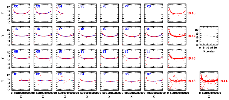
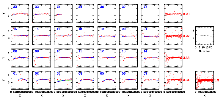
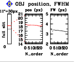
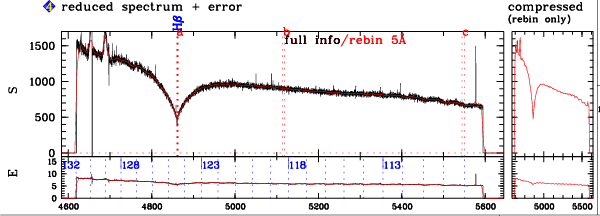
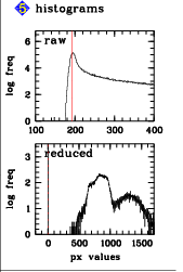
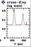
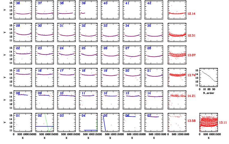
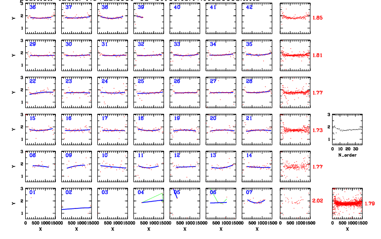
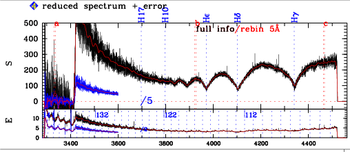
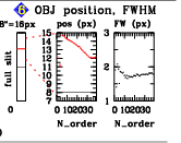
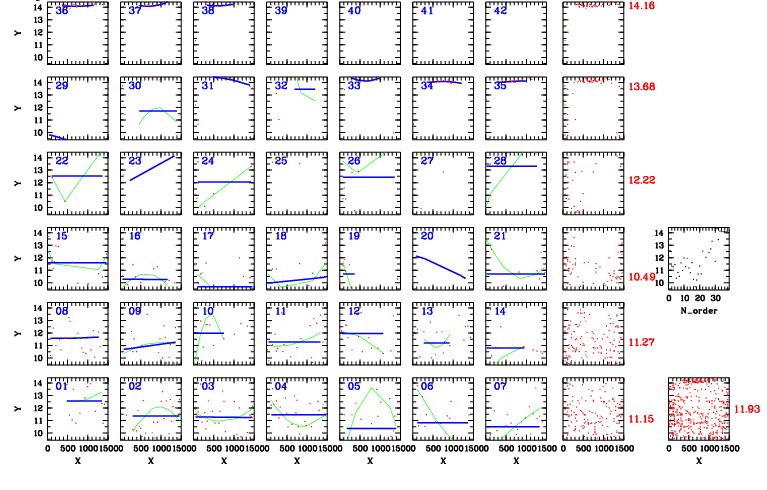
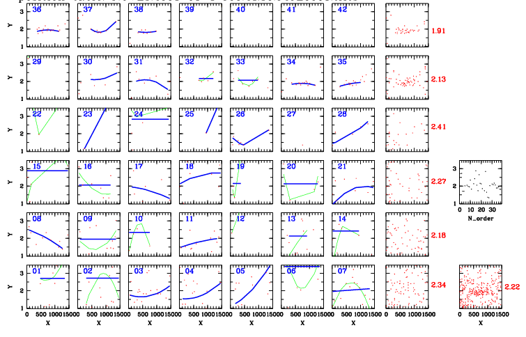
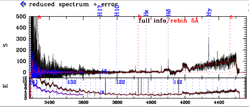
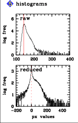
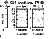
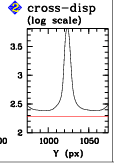
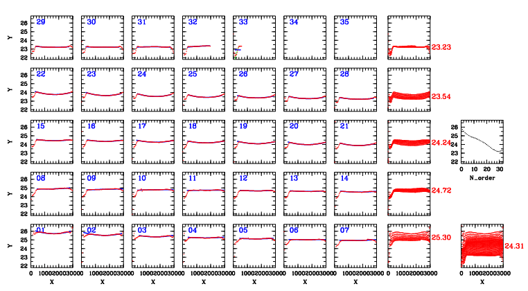
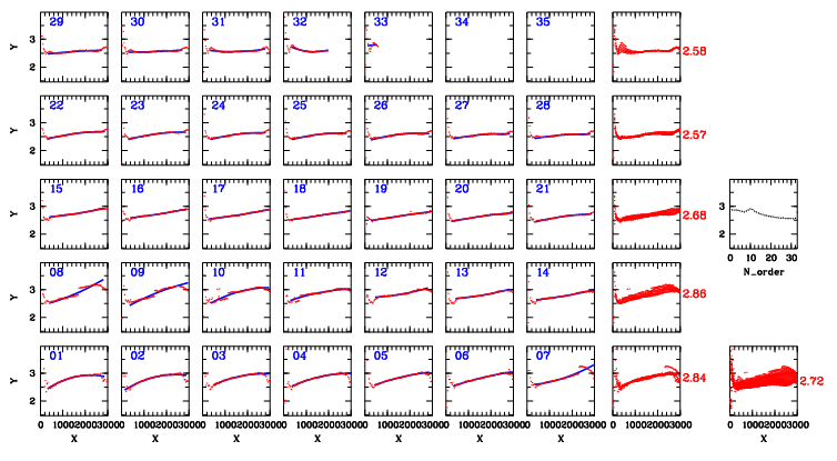
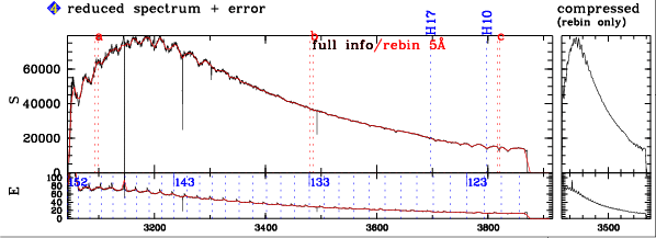
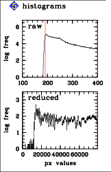
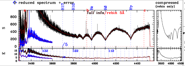
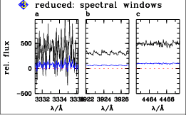
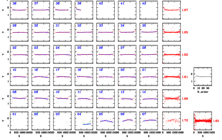
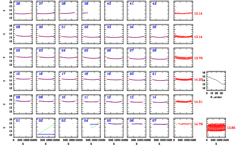
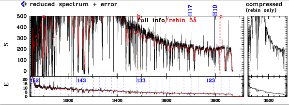
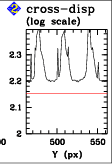
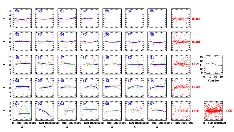
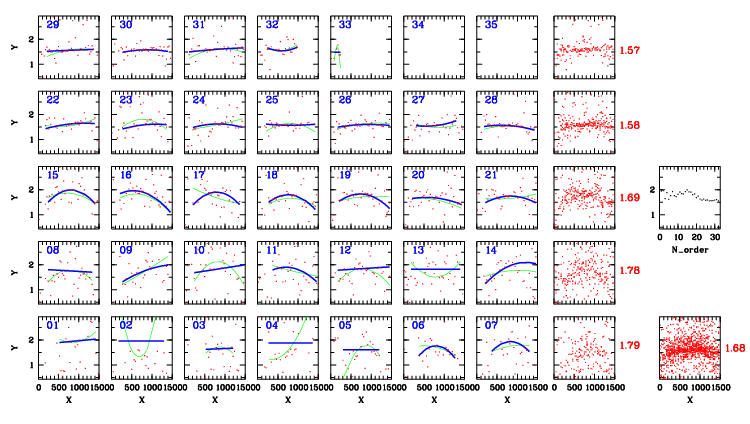
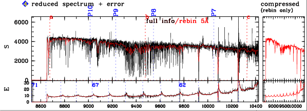
The position plot of a properly extracted spectrum shows a close match of red points and blue curve in all orders. Generally the tracing is very reliable if the rms scatter of the red dots is smaller than the curvature of the blue curve. The example shown here is a red spectrum. The summary plots (rightmost columns) show a consistent behaviour. The mean position per order is almost constant.

The FWHM plot confirms this. The fitting routine is mostly stable against outliers. The summary plots show an almost constant width per order. This is also visible in the box 6 plot.

The extracted spectrum is smooth. The position and FWHM plots show that the extraction routine is, e.g., stable against the steep flux drop around H beta (order no. 8). The histogram plot (raw data) shows the typical shape of a well-exposed spectrum: maximum around the bias value, with a long and slowly (on a log scale) decreasing tail. The cross-dispersion profile (box 2) has a well-pronounced peak.

The position plot shows a characteristic increase towards the left. This increase, though not matched by the fit, is not critical as long as there is sufficient overlap of spectral coverage in the orders.

Airmass too high (blue spectra affected)

The main effect of high airmass on the extraction quality is atmospheric dispersion. In spectra taken without atmospheric dispersion compensation, the object is found off-center (since centering is done on the red acquisition CCD) and in addition differentially shifted, against the mean position. Both effects together can act to shift the signal out of the extraction window for certain orders. Typically such behaviour is observed at airmass > 1.4, for the bluemost orders. Due to the strong dependency of differential dispersion on wavelength, this effect is generally unimportant for red spectra.

The example shown here is from a well-exposed blue spectrum (setting 390_DI2_2x2) taken at airmass 1.9. The position plot shows that the extraction routine has failed in the first 6 orders. The nominal slit center is at Y = 8 px while the signal in order 7 is almost at 15 px, and is found at Y = 8 in the last order of the example, N = 38.

Both the slight curvature of the signal and its inclination within an order (both by several 0.1 pixels) are not critical since the algorithm uses a 2nd order polynomial fit. The summary plots in column 9 clearly show the strong effect of differential dispersion, together with the loss of the signal in the first orders.

With no significant points left in the first 6 orders, the plotted fit results are meaningless.

The FWHM plot shows the same result. Since the positions for the first orders are wrong, the fitted width values have no meaning. Once the proper positions are found, the width values are 'in resonance' again. This becomes clearly visible in the summary plot, with the initial scatter and the almost constant values for order numbers > 6.

The spectrum (preview extracted from box 4 in the complete SCIENCE QC1 report) shows the failure in the first orders clearly. The diagnosis is also clearly visible in box 6 with the nominal slit center and the average true position found.

Note that the 390 settings always have the spectrum plotted twice, with a scaled version in blue (scaling factor is 5 for the spectrum, and 2 for the errorbars).

Occurrence. Blue settings at airmass ~1.4 or higher.

Solution. A priori: observe at lower airmass, use ADC; a posteriori: none; maybe: use average extraction.

Flux too low

The UVES pipeline has no "insufficient flux alarm" so it will always give an extraction result (provided that all calibration data are present and the science frame is nominally intact, i.e. has no problems with the FITS header). It is therefore important to know how unsuccessful extraction of a spectrum (or parts thereof) can be easily recognized.

The position plot shows that the positions (both found and fitted) are just random, except for the very last ones. The same is true for the FWHM values. Therefore, the extracted spectrum does not contain useful information, any features found are not significant. The only exception are the very last orders (beyond 34) where the pipeline has found a signal. The box 5 plot (histogram) confirms that almost no flux has been extracted (the histogram of the reduced data is almost symmetric around 0). The box 6 plot shows once more the scatter in the average positions and FWHM found.

Occurrence. Potentially in all settings.

Solution. A priori: use longer exposure times. A posteriori: none; if you have reasons to believe there is a faint signal, try to use average extraction.

Flux too high

In the pipeline/optimum extraction sense, a spectrum (or parts thereof) have too high a flux if the instrumental profile in cross-dispersion direction deviates from a Gaussian. This includes the case of over-exposure (where the top part of the signal would ramp off) but clearly starts to show up at much lower levels. The example shown here has almost 10.000 ADU in the raw data (see box 2).

The position plot is very smooth. Hardly any rms deviations between measured positions and the final fit are visible. However, there are systematic effects, namely the measured positions have a steep initial step which the fit cannot follow. It is a defining property of this problem that systematic effects dominate random scatter.

The FWHM plot shows the same characteristics. As a result, the extraction algorithm looses part of the flux at the borders of the orders, because both the width and the positions used in the fit are systematically wrong. Furthermore, this effect is increased by the inclination of the FWHM across an order which is untypically high and again indicative for a non-Gaussian flux profile.

This results, in the extracted spectrum, in a ripple-like pattern which repeats with the period of the orders (clearly visible in the compressed part of the plot, and also in the errorbar plot). This pattern is very typical. While it affects the spectral shape in general, it does generally not disturb on smaller scales (however, see small-scale ripples).

The high level of exposure is also visible in the raw data histogram as flat slope.

Occurrence. Since the orders are narrowest in the blue, this problem typically affects the bluemost spectra (settings 346 and 390).

Solution. A priori: avoid such high exposure levels. A posteriori: use average extraction here which makes no assumption on the flux profile and may give better results here.

Small-scale ripples

Occasionally there are cases when the optimum extraction introduces small-scale ripples, contrary to the "flux too high" problem. An example is shown here. While the extracted spectrum suffers from the "airmass too high" problem, there is an additional effect best visible in the three spectral closeups (box b). The extracted flux has a small-scale ripple pattern which increases the noise and may work against line identification, profile studies etc. Its origin becomes apparent in the width plot (and to a lesser degree in the position plot).The initial ~25 orders have the measured widths (red dots) ondulating around the fitted widths (blue line). Since this is a systematic effect, a small amount of extracted flux is lost with the period of the ondulation and creates the ripples.

The period is presumably caused by the CCD pixel grid and due to some instability of the optimum extraction algorithm to the inclination of the echelle orders. With pipeline version 1.2, this effect has become much reduced but it is sometimes still there.

Occurrence. Rarely, in the blue spectra.

Solution. Maybe average extraction gives better results.

Extended source

Extended sources by definition violate one of the underlying assumption for the optimum extraction properly working, namely having an unresolved, point-like flux distribution. In case any structure in the source, the order tracing mechanism may run crazy and obtain odd results. This may become apparent in the position and/or width plots only.

As an example, the following spectrum is from an extended source. The extracted spectrum does not show any peculiarity. The cross-dispersion flux profile is complex, however, and clearly non-point like. This is supported by the position and width plots. Both show a large scatter, which is not due an insufficient flux level. The position plot even shows indications of a bifurcation (second and third row, summary plots). Furthermore the mean FWHM value (0.85 arcs) is much higher than the seeing (0.48 arcs) also indicating a resolved source structure.

Occurrence. Any setting.

Solution. No complete UVES pipeline reduction is available for extended sources. The 2D extraction mode may help in constructing the reduction solution.

Spectral gaps

The redmost settings have spectral gaps since the echelle orders do not overlap anymore. While this is due to the spectral format and therefore beyond influence of the user, it may be useful to know how this effect looks like in the extracted spectra. In the 860 setting, the gaps show up beyond 9700 A. In the example shown here, the gaps are clearly visible in the errorbar plot, at the position of the blue broken lines, between the last four orders. Once these positions are known from the errorbar file, they are easily found in the extracted spectra.

Occurrence. Redmost settings, beyond 9700 A.

Solution. None.