3.2 SPATIAL DISTRIBUTION

3.2.1 IMAGING

1. Total magnitude in one of the associated broad band filters. It is assumed that the total light coming from the source falls inside a circle of radius = ImageQualityFWHM.

1. Mean surface brightness in mag/arcsecs ² again in one of the associated filters.

1. Aperture magnitude (mag) they want to reach.
2. Aperture radius (arcsecs).

3.2.2 MOS SPECTROSCOPY

1. Magnitude (mag/arcsecs ²) in one of the associated broad band filters. For De Vaucouleurs and Exponential profiles, this is intended as the central surface brightness.
2. Surface brightness distribution.
3. Projected semi-major axis.

3.2.3 IFU SPECTROSCOPY

3.3 ATMOSPHERE

• Airmass.
• Seeing.

Sky Conditions

• Turbulence Category (T category)

  With the advent of instruments using new adaptive optics (AO) modes, new turbulence parameters need to be taken into account in order to properly schedule observations and ensure that their science goals are achieved. These parameters include the coherence time and the fraction of turbulence taking place in the atmospheric ground layer, in addition to the seeing. Starting from Period 105, the turbulence constraints are standardised to the turbulence conditions required by all instruments and modes, whether they are seeing-limited or AO-assisted.

  The handling of atmospheric constraints thus changes for both Phase 1 (proposal preparation) and Phase 2 (OB preparation). In Phase 1, the seven current seeing categories are replaced by seven turbulence categories for all instruments. Each category can be defined by other parameters than a pure seeing threshold, depending on the instrument. For all instruments, all categories share the same statistical probability of realisation, which is key for an accurate time allocation process. In Phase 2, the image quality will still be the only applicable constraint for seeing-limited modes, whereas the same turbulence category as for Phase 1 will be used for diffraction-limited modes.

  Users are encouraged to read the general description of these changes for Phase 1 and Phase 2 on the Observing Conditions webpage, as well as instrument User Manuals for specifics per instrument.

  Seeing and Image Quality

  The definitions of seeing and image quality used in the ETC follow the ones given in Martinez, Kolb, Sarazin, Tokovinin (2010, The Messenger 141, 5) originally provided by Tokovinin (2002, PASP 114, 1156) but corrected by Kolb (ESO Technical Report #12): Seeing is an inherent property of the atmospheric turbulence, which is independent of the telescope that is observing through the atmosphere; Image Quality (IQ), defined as the full width at half maximum (FWHM) of long-exposure stellar images, is a property of the images obtained in the focal plane of an instrument mounted on a telescope observing through the atmosphere. The IQ defines the S/N reference area for non-AO point sources in the ETC. With the seeing consistently defined as the atmospheric PSF FWHM outside the telescope at zenith at 500 nm, the ETC models the IQ PSF as a gaussian, considering the gauss-approximated transfer functions of the atmosphere, telescope and instrument, with s=seeing, λ=wavelength, x=airmass and D=telescope diameter: Image Quality \( { \begin{equation} \mathit{FWHM}_{\text{IQ}} = \sqrt{\mathit{FWHM}_{\text{atm}}^2(\mathit{s},x,\lambda)+\mathit{FWHM}_{\text{tel}}^2(\mathit{D},\lambda)+\mathit{FWHM}_{\text{ins}}^2(\lambda)} \end{equation} } \) For fibre-fed instruments, the instrument transfer function is not applied. The diffraction limited PSF FWHM for the telescope with diameter D at observing wavelength λ is modeled as: \( \begin{equation} \begin{aligned} \mathit{FWHM}_{\text{tel}} & = 1.028 \frac{\lambda}{D} \text{, } & \text{ with } \lambda \text{ and D in the same unit}\\ & = 0.000212 \frac{\lambda}{D} \text{arcsec, } & \text{ with } \lambda \text{ in nm and D in m}. \end{aligned} \end{equation} \) For point sources and non-AO instrument modes, the atmospheric PSF FWHM with the given seeing \(s\) (arcsec), airmass \(x\) and wavelength \({ \lambda }\) (nm) is modeled as a gaussian profile with: $${\mathit{FWHM}}_{\text{atm}}(\mathit{s},\mathit{x},\lambda) = \mathit{s} \cdot x^{0.6} \cdot (\frac {\lambda} {500})^{-0.2} \cdot \sqrt{[1+F_{\text{Kolb}} \cdot 2.183 \cdot ({r_0}/L_{0})^{0.356})]}$$ Note: The model sets \({ \mathit{FWHM}}_{\text{atm}}\)=0 if the argument of the square root becomes negative \({ [1+F_{\text{Kolb}} \cdot 2.183 \cdot ({r_0}/L_{0})^{0.356}] < 0 }\) , which happens when the Fried parameter \({ {r_0} } \) reaches its threshold of \({ r_{\text{t}} = L_{0} \cdot [1/(2.183 \cdot F_{\text{Kolb}})]^{1/0.356}}\). For the VLT and \({ L_{0} = 46m}\) , this corresponds to \({ r_{\text{t}} = 5.4m} \). \({ L_{0} }\) is the wave-front outer-scale. We have adopted a value of \({ L_{0} }\)=46m (van den Ancker et al. 2016, Proceedings of the SPIE, Volume 9910, 111). \(F_{\text{Kolb}} \) is the Kolb factor (ESO Technical Report #12): $$F_{\text{Kolb}} = \frac {1}{1+300 {\text{ }} D/L_{0}}-1$$ For the VLT and \({ L_{0} }\)=46m, this corresponds to \(F_{\text{Kolb}} = -\)0.981644. \( {r_0} \) is the Fried parameter at the requested seeing \(s\), wavelength \({ \lambda }\) and airmass \(x\): $$r_0 = 0.100 \cdot s^{-1} \cdot (\frac{\lambda}{500})^{1.2} \cdot x^{-0.6} \text{ m, } \text{ } \text{ } \text{ } \text{ with } s \text{ in arcsec } \text{and } \lambda \text{ in nm.} $$

  For AO-modes, a model of the AO-corrected PSF is used instead.

  
  

  Sky Model

  The sky background model is based on the Cerro Paranal Advanced Sky Model, also for instruments at la Silla, except for the different altitude above sea level. The observatory coordinates are automatically assigned for a given instrument.
  

  Almanac

  By default, the airmass and moon phase parameters are entered manually. The sky model will use fixed typical values for all remaining relevant parameters (which can be seen in the output page by enabling the check box "show skymodel details").

  Alternatively, a dynamic almanac widget can be enabled to facilitate assignment of accurate sky model parameters for a given target position and time of observation. The sky radiation model includes the following components: scattered moonlight, scattered starlight, zodiacal light, thermal emission by telescope and instrument, molecular emission of the lower atmosphere, emission lines of the upper atmosphere and airglow continuum.

  The almanac is updated dynamically by a service on the ETC web server, without the need to manually update the web application.

  Notes about the algorithms, resources and references for the almanac are available here. A more advanced version of the almanac is included in our SkyCalc web application, which provides more input and output options.

  Hovering the mouse over an input element in the almanac normally displays a pop-up "tooltip" with a short description.

  Time

  The upper left part of the almanac box refers to the date and time of observation.
  This can be done with a UT time or a MJD. A date/time picker widget will appear when the UT input field is clicked, but the UT can also be assigned manually. In any case, the UT and MJD fields are dynamically coupled to be mutually consistent.

  The two +/- buttons can be used to step forward or backward in time by the indicated step and unit per click. The buttons can be held down to step continuously until released.

  The third of night corresponding to the currently selected time is indicated. This is an input parameter to the airglow component in the sky model. Twilight levels (civil, nautical and astronomical) referring to the sun altitude ranges are also indicated in the dynamic text. These levels refer to the sun altitude:

  • Astronomical Twilight −18^° ≥ alt_☉ < −12^°
  • Nautical Twilight −12^° ≥ alt_☉ < −6^°
  • Civil Twilight −6^° ≥ alt_☉ < 0^°

  Target

  The target equatorial coordinates RA and dec can be assigned manually in the two input fields or automatically using the SIMBAD resolver to retrieve the coordinates.
  If the lookup is successful, an "info" link will open a window in which the raw SIMBAD response can be inspected.
  The units can be toggled between decimal degrees and hh:mm:ss [00:00:00 - 23:59:59.999] for RA and dd:mm:ss (or dd mm ss) for dec. A whitespace can be used as separator instead of a colon.

  Output Table

  The table dynamically displays the output from the server back-end service, including temporal and spatial coordinates for the target, Moon and Sun. The bold-faced numbers indicate the parameters normally relevant in the phase 1 proposal for optical instruments. The numbers appear in red color if they are out of the range supported by the sky model.

  Visiblity Plot

  The chart dynamically shows the altitude and equivalent airmass as function of time for the moon and target, centered on midnight for the currently selected date.
  The green line, which refers to the currently selected time, can be dragged left and right to change the time, dynamically coupled with the sections in the Time section.

  3.4 OPTICAL PATH

  3.4.1 IMAGING

  Requested parameters:
  
  1. Filter.
  2. Detector read mode slow.
  3. Binning.
  
  

  3.4.2 MOS SPECTROSCOPY

  Requested parameters:
  
  1. Grism name.
  2. Slit dimensions (length = spatial direction, width = dispersion direction) in arcsec.
  3. Detector read mode slow.
  4. Binning.
  
  
  The various order sorting filters are automatically loaded once you have selected the grism.
  
  Choosing a long slit requires more computational time for the source profile (which is computed along the whole slit), especially for extended sources, for which both the PSF and the surface brightness profiles must be evaluated, and convolution is applied.
  
  
  

  3.4.3 IFU SPECTROSCOPY

  Requested parameters:
  
  1. Grism name.
  2. IFU spatial sampling factor.
  3. Detector read mode slow.
  4. Binning.
  
  

  3.5 OBSERVATION

  This part of the input form is common to all the observing modes.
  
  Here the user can choose between:
  
  1. Given the S/N (intended as the one per pixel at grism central wavelength for the spectroscopic case), compute the requested Exposure Time.
  2. Given the Exposure Time, compute the S/N (intended as the S/N per pixel one would reach at grism central wavelength for the spectroscopic case).
  
  
  Other parameters are:
  
  3) Fractional flat-field accuracy.This is currently set to 0.0 until empirical values are known
  
  4) Optional: S/N or Exposure Time range.
  
  
  
  Note that for spectroscopy the reference wavelength is always the grism central wavelength.
  
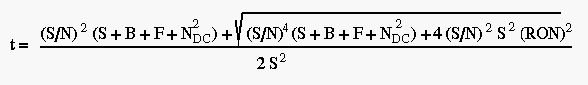
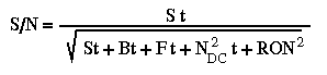
  Ranges for exposure time and S/N are used to evaluate S/N as a function of exposure time: see the graphical outputs below. If you leave the fractional flat-field accuracy to zero, this term is not taken into account in S/N computations (see the formulae in Section 2.1).

  
  

  4. ETC COMPUTATIONS

  In this section we describe the various computations made by the ETC. The first step, common both to imaging and spectroscopic modes, consists in initializing the model. Different computations performed by the various observing modes are described in Section 4.2 and following.
  

  
  

  4.1 INITIALIZING THE MODEL

  a) Instrument setup: starting from your choice of instrument setup, a "simulated" instrument is built with the proper optical components.
  

  
  

  c) Source: according to the user choice, a source spectrum is built. Redshift the spectrum (only for User Defined and From List SEDs).
  

  
  

  d) Scale source template spectrum accordingly to magnitude
  

  
  

  e) Scale sky spectrum accordingly to sky brightness. This is done by scaling a template spectra of the sky (including emission lines) to a certain magnitude.
  

  
  

  Maths:
  

  1) Redshifting (optional).
  

  For each lambda in the input spectrum do:
  

  
  

  LambdaNew = (LambdaOld * Redshift) + LambdaOld
  

  IntensityNew = IntensityOld / (1 + Redshift)
  

  
  

  Where LambdaOld, IntensityOld are rest frame.
  

  
  

  2) Magnitude scaling. Once selected the band and zero-point f do:
  

  
  

  logFlux = -0.4 * Magnitude + Log ₁₀ (f)
  

  Flux = 10 ^(logFlux)
  

  
  

  Then, scale the source spectrum so to have this flux at the filter central lambda. The same operation is done for the sky spectrum.
  

  
  

  NOTE: because of some problems in the WucSpectralTarget class that handles the input flux distributions, except for Flat Spectrum currently the scaling is done at the filter central lambda; integration and normalization under the filter "profile" is not implemented yet.
  

  
  

  4.2 IMAGING MODE: TRANSFORMING THE MODEL

  4.2.1 System efficiency

  a) Create system efficiency for source: atmosphere + telescope + instrument
  

  b) Create system efficiency for sky: telescope + instrument
  

  
  

  Instrument overall efficiency is evaluated as a function of lambda. Its intensity is the combination of the efficiencies of each single component and its wavelength range is the resultant bandpass of the instrument for that observational setup.
  

  
  

  Maths:
  

  1) A tmospheric extinction (source only).
  

  Atmospheric extinction is applied at each lambda in the source spectrum, by means of the formula:
  

  
  

  Intensity(Lambda) = Intensity(Lambda) * 10 ^{(-0.4 * Extinction(lambda) * Airmass)}
  

  
  
  Components acting (also) like filters are: telescope mirror, photometric filters, lenses, detector (QE). For each component acting like a filter, do:
  
  
  
  Efficiency(Lambda) = Efficiency(Lambda) * Table(Lambda)
  
  
  
  Where, for each component, "Table" is its tabulated transmission. Tabulated values are read and transformed to a continuous function 1D, to interpolate missing values.
  
  
  

  4.2.2 Going to Counts: Effective Area and Detector

  a) Conversion from erg/sec/cm ²/A to photo-electrons/sec is performed at each lambda in the spectrum.
  
  b) Wavelength integration is done over the sky and source spectrum.
  
  c) Pointlike sources and integral photometry: source and sky signals are multiplied by the telescope effective area. Sky signal is multiplied by the number of pixels in a PSF area as well.
  
  d) Extended sources: source and sky signals are multiplied by the telescope effective area and the pixel size.
  
  
  
  Units are now: e-/sec for pointlike sources and integral photometry options.
  
  e-/sec/pixel for extended sources.
  
  Source and sky counts are then used to apply the formulae in Section 2.1 for S/N and Exposure Time calculation.
  
  
  
  Maths:
  
  1) Conversion to photons. At each wavelength in the spectrum do:
  
  
  
  Intensity(Lambda) = Intensity(Lambda) * Lambda / (h * c)
  
  
  
  Where:
  
  c = 2.9979 x 10 ¹⁸ [A/s]
  
  h = 6.6262 x 10 ^-27 [erg s]
  
  
  
  2) Effective area and Detector.
  
  
  
  LensSurface = π * [ (Mirror_Radius) ² : (Centr_Obstr_Radius) ² ]
  
  
  
  - Pointlike sources:
  
  source: Intensity = Intensity * LensSurface
  
  sky: Intensity = Intensity * LensSurface * arcsecs ² * npsf
  
  Where npsf = (π * ImageQualityFWHM ² ) / (arcsecs ² )
  
  
  
  - Extended sources:
  
  source and sky: Intensity = Intensity * LensSurface * arcsecs ²
  
  
  
  - Integral photometry:
  
  source: Intensity = Intensity * LensSurface
  
  sky: Intensity = Intensity * LensSurface * arcsecs ² * n_aper
  
  Where n_aper = (π * aperture_radius ² ) / arcsecs ²
  
  
  

  4.3 SPECTROSCOPIC MODE: TRANSFORMING THE MODEL

  In this Section we describe the computations performed by the spectroscopic ETC. Unless explicitly specified in Section headings, the following steps are applied both to IFU and MOS modes.
  
  Starting from the source and sky spectra normalized to observed magnitude, the first two steps are the evaluation of the overall system efficiency and of the dispersion relation.
  
  
  

  4.3.1 System efficiency

  See Section 4.2.1. Here the components acting like filters are: telescope mirror, grism and order sorting filter, lens, detector (QE).
  
  For IFU spectroscopy, the microlens+fiber etc. etc. are considered as well. When the user selects IFU high resolution (spatial sampling 0.3 arcsecs per fiber), the focal elongator transmission is also included.
  
  
  

  4.3.2 Dispersion relation

  This step evaluates the geometrical transformations, i.e. grism and lens. These transformations act only on directional angles and not on intensity. Look at each "photon" in the spectrum as an optical ray entering the system with directional angles inAlpha =0; inGamma = 0 (Alpha = atan (Y), Gamma = atan (X).
  
  Gamma angle (X direction) is not affected by dispersion/geometrical transformations in this model.
  
  
  
  a) Determine dispersion relation for the given grism: its angular dispersion and lambda_c are used to determine the number of nm/pixels at each pixel on the detector. It is a linear relation.
  
  
  
  Maths:
  
  1) Grism. The grism is treated as a dispersing element.
  
  Each optical ray enters the system with (inAlpha=0,inGamma=0) directional angles.
  
  For each lambda in the spectrum, do:
  
  
  
  outAlpha = inAlpha + ((Lambda - Lambda_c) * mDisp)
  
  (outGamma = inGamma)
  
  
  
  Where Lambda_c = grism central wavelength and mDisp is the grism angular dispersion.
  
  Angular dispersion for each grism is evaluated as:
  
  
  
  A = 1 / (f _camera * P)
  
  
  
  Where P is the reciprocal linear dispersion and f _camera the Camera focal length.
  
  
  
  2) Lens. The optical ray now enters the lens with inAlpha ≠ 0.
  
  For each lambda do:
  
  
  
  y = tan(inAlpha) * fy
  
  outAlpha = atan(y)
  
  (outGamma = inGamma)
  
  
  
  Where fy is the focal length of the instrument, given by:
  
  
  
  fy = (pixel size [cm] ) / (plate scale [radians] )
  
  
  

  4.3.3 Apply efficiency and dispersion relation to source and sky spectra

  System efficiency and dispersion relation are applied to the source spectrum: we obtain a new spectrum, with now intensity expressed as a function of pixel. The same holds true for the sky spectrum.
  
  
  
  Maths:
  
  1) Transformed intensity.
  
  From the dispersion relation we know skyProjection = dispersion at central pixel, i.e. the number of Angstroms per pixel at the central position (which : given the dispersing characteristics of this model - corresponds to the grism central lambda)
  
  At each pixel yp along dispersion direction do:
  
  
  
  yp = pixel_size * (mw - Lambda_c) / skyProjection
  
  factor = (Efficiency(mw)) * dispRelation(yp)
  
  Intensity(yp) = Intensity(Lambda) * factor
  
  
  
  Where yp is the pixel coordinate, pixel_size is the linear size of the pixel, mw is the wavelength corresponding to the pixel yp (due to dispersion), Lambda_c is the grism central wavelength.
  
  The dispersing element is defined as the range in lambda covered by one pixel at Lambda_c, thus this range is affected by the pixel size which, in turns, is affected by the detector binning.
  
  By means of the term "factor" we integrate the signal over one dispersing element.
  
  
  

  4.3.4 Slit PSF

  We need now to build the slit PSFs for source and sky: these are used for convolution of source and sky spectra along the dispersion direction. Refer to these as the PSFs along the dispersion direction (= slit PSFs). Later we will define the PSFs along the spatial direction for spectroscopy.
  
  
  
  a) Source: a gaussian profile with radius = ImageQualityFWHM is defined from (- slitWidth/2) to (+ slitWidth/2) and its area is normalized to unity.
  
  
  
  b) Sky: a "flat" profile is built from (- slitWidth/2) to (+ slitWidth/2). The transmission of this profile is the same at each position, and the area is again normalized to unity.
  
  
  
  c) Convolution of the spectra with their associated slit PSFs is done
  
  
  
  For IFU, the slit width is set equal to the IFU pseudoslit size along the dispersion direction, which is about 1".
  
  
  
  Maths:
  
  1) Slit PSF for source and sky.
  
  For each sampling interval i across the slit do:
  
  
  
  x(i) = slit_start + arcsecs * i
  
  
  
  Define the gaussian sigma: s_sigma = ImageQualityFWHM / 2.35482
  
  PSF_source(i) = [ exp(- x ² / (2 * s_sigma ² )) / (sqrt(2 * π * s_sigma) ] / norm1
  
  
  
  PSF_sky(i) = [1 / (2 * n_sample + 1) ] / norm2
  
  
  
  Where n_sample is the number of sampling intervals across slitWidth, norm1 and norm2 are the area normalization factors, and arcsecs is the plate scale (0.205").
  
  
  

  4.3.5 MOS: going to Counts

  In the following subsections we describe the computations necessary to evaluate source and sky counts in MOS observing mode.
  

  4.3.5.1 Slit losses : Pointlike sources only

  Slit losses are computed by integrating the slit PSF over the slitWidth.
  
  
  
  Maths:
  
  1) Slit transmission.
  
  
  
  slit_trans = erf [ (slitWidth / 2) / sqrt(2.) * s_sigma ];
  
  
  
  The erf function comes from Math Library. The output parameter "Slit Losses" is (1 - slit_trans).
  

  4.3.5.2 Effective Area and Detector

  a) Conversion from erg/sec to photo-electrons/sec is performed.
  
  b) Pointlike sources: counts coming from the source are integrated over the telescope effective area and multiplied by slit losses.
  
  c) Extended sources: counts coming from the source are integrated over the telescope effective area, over the solid angle of the source (slitWidth), and over pixel size in arcsec. We are assuming that in the dispersion direction the source dimension is greater or equal to the slitWidth.
  
  
  
  Maths:
  
  1) Conversion to photons. At each pixel yp do:
  
  
  
  Intensity(yp) = Intensity(yp) * mw /(h * c)
  
  
  
  Where mw is the lambda corresponding to pixel yp, and c and h are defined in Section 4.2.2.
  
  
  
  2) Integration.
  
  
  
  - Pointlike sources . At each pixel do:
  
  Intensity = Intensity * LensSurface * slit_trans
  
  
  
  - Extended sources . At each pixel do:
  
  Intensity = Intensity * LensSurface * slitWidth * arcsecs
  
  
  
  Where lensSurface is same as in Section 4.2.2.
  
  
  
  At this point, we have: source and sky spectra as seen through VIMOS. These are 1D spectra, with lambda sampled at each pixel along the CCD.
  
  Units: (e-/sec) for pointlike sources;
  
  (e-/sec/pixel) for extended sources.
  
  In MOS spectroscopic case, before evaluating S/N we need a further step in the spatial direction.
  

  4.3.5.3 Spatial Direction

  Pointlike sources
  
  The flux we see at each lambda in the spectrum is the TOTAL one (we assume the total light inside a circle of radius ImageQualityFWHM). The "spatial" PSF (i.e. along X direction) is computed along the slit, and its area is normalized to unity. This is necessary not only to generate the simulated image, but especially because - as the sky is given as [e-/sec pixel] - we need to know how many pixels are inside the 2*ImageQualityFWHM length, to compute sky signal inside a PSF diameter. The computations for spatial PSF are similar to those for the slit PSF, except that now we use slitLength instead of slitWidth.
  
  
  
  Extended sources
  
  Hereafter: SBP = surface brightness profile.
  
  a) Take the SBP curve, symmetric around the central pixel and sampled at each pixel along the slit, i.e. define it each 0.205" from (- slitLength / 2) to (+ slitLength / 2). The slit center coincides with the profile center.
  
  b) Apply pixel subsampling (we use subsampling factor = 11).
  
  c) Normalize the SBP so that its intensity over the central pixel is =1.
  
  d) Take the spatial PSF and subsample it.
  
  e) Convolution of the SBP with the PSF along the slit.
  
  f) Rebin the SBP so to have again 1 sampling per pixel.
  
  
  
  Now we have the final spatial profile: its value at the central pixel is no more equal to 1, due to convolution.
  
  Here we determine also the output parameter "Intensity factor (spatial summing)" and the central pixel intensity factor that will be used to evaluate S/N over the central pixel. See below for details.
  
  
  
  NOTE: convolution is applied also to uniform brightness profile, in order to smooth the SBP at its edges along the slit.
  
  
  
  Maths:
  
  1) Profiles.
  
  For each x position along the slit do:
  
  
  
  De Vaucouleurs: Intensity[i] = exp( (-7.67) * [ (x[i]) / r_eff) ^0.25 ]
  
  
  
  Exponential: Intensity[i] = exp ( -1.6783 * [ (x[i]) / r_eff) ]
  
  
  
  Uniform: if (x[i] >= -r_eff or x[i] <= r_eff) Intensity[i] = 1.
  
  If (x[i] < -r_eff or x[i] > r_eff) Intensity[i] = 0.
  
  
  
  Where r_eff is the effective radius in arcsecs. The number of points, i, is defined by slitLength and subsampling factor.
  

  4.3.5.4 Counts

  Pointlike sources
  
  As already said, all the flux we see at each lambda in the spectrum comes from the TOTAL source (we assume the total light inside a circle of radius ImageQualityFWHM), i.e. we already have source counts. The sky counts (in e-/sec/pixels) are multiplied by the number of pixels in a PSF diameter, to get the total sky contribution.
  
  
  
  Extended sources
  
  Source and sky signal must be summed over 2*r_eff along the slit.
  
  a) The SBP is the observed (i.e. transformed by the instrument + atmosphere etc. etc.) spatial intensity distribution of the source. If we sum the profile values from -r_eff to +r_eff, we know the fraction of flux falling inside (-r_eff, +r_eff): this number is the "Source: Intensity factor" parameter in the numerical output for extended sources.
  
  Having the source spectrum, which is still normalized to the central surface brightness outside atmosphere, if we multiply the spectral intensities at each lambda by this "intensity factor", we have the (e-/sec) source counts integrated over (-r_eff, +r_eff) along the slit.
  
  Sky counts are multiplied by the number of pixels in (-r_eff, +r_eff). This number is referred as " Sky n. of pixels (spatial summing )" in the numerical output.
  
  
  

  4.3.6 IFU: going to Counts

  In the following subsections we describe the computations that are done to evaluate source and sky counts in the IFU observing mode. In IFU observing mode, source and sky counts are computed in a different way with respect to MOS mode.
  
  After entering the IFU head, each source is seen as a pointlike one, and what "dominates" from the IFU head onward is the fiber shape. What enters the spectrograph is the total light collected by one microlens (extended sources) or by all the microlenses covering the source (pointlike sources) and each source is "seen" as a pointlike one.
  
  When dealing with extended sources and sky, the signal entering the IFU head is first integrated over a fiber area and no more referred to square arcsecs. For pointlike sources, we again assume the total light inside a circle of radius ImageQualityFWHM and compute the number of fibers receiving signal from the source. Both for sky and source, the flux at each lambda in the spectrum is the TOTAL one coming from 1 fiber.
  

  4.3.6.1 Effective Area and Detector

  a) Conversion from erg/sec to photo-electrons/sec is performed.
  
  We consider the microlens area as a square one.
  
  b) Pointlike sources: counts coming from the source are integrated over the telescope effective area. It is assumed that the signal from all the fibers covering the source is summed to obtain a single spectrum. The sky signal (mag/square arcsec) is first integrated over the area of 1 microlens, and then multiplied by the number of fibers covering the pointlike source.
  
  c) Extended sources: counts coming from the source are integrated over the telescope effective area and over 1 fiber area. The same is done for sky counts: in this case N _fib is defaulted to 1.
  
  
  
  Maths:
  
  1) Conversion to photons. At each pixel yp do:
  
  
  
  Intensity(yp) = Intensity(yp) * mw /(h * c)
  
  
  
  Where mw is the lambda corresponding to pixel yp, and c and h are defined in Section 4.2.2.
  
  
  
  2) Integration.
  
  
  
  - Fiber area:
  
  A_fib = (spatial_sampling) ²
  
  
  
  - Number of fibers covering the source:
  
  N_fib = (PI * (seing) ² ) / A _fib
  
  
  
  Where the IFU spatial sampling can be 0.33" or 0.66".
  
  
  
  - Pointlike sources . At each pixel do:
  
  source: Intensity = Intensity * LensSurface
  
  sky: Intensity = Intensity * LensSurface * A _fib * N _fib
  
  
  
  - Extended sources . At each pixel do
  
  source: Intensity = Intensity * LensSurface * A _fib
  
  sky: Intensity = Intensity * LensSurface * A _fib
  
  
  
  Where LensSurface is as in Section 4.2.2.
  
  
  
  At this point, we have: source and sky spectra as seen through VIMOS. These are 1D spectra, with lambda sampled at each pixel along the CCD.
  
  Units: (e-/sec) both for pointlike and extended sources.
  

  4.3.6.2 Spatial Direction

  As mentioned above, after having entered the IFU head, we loose track of the source morphology, that is the signal is a total one (integrated over a fiber area when needed) and no more referred to square arcsecs. The flux we see at each lambda in the spectrum is the TOTAL one (we assume the total light inside a circle of radius ImageQualityFWHM). The "spatial" PSF (i.e. along X direction) is computed along the slit, and its area is normalized to unity. This is necessary to generate the simulated image. The computations for spatial PSF are similar to those for the MOS slit PSF, except that now slitLength is fixed by the characteristics of IFU slits. Each fiber "produces" on the IFU mask a pseudoslit whose dimensions (slitWidth and slitLength) are equivalent to about 1". Thus, CCD for one IFU pseudoslit we fixed the number of pixels in the spatial direction on the to be 5.
  
  
  

  4.3.7 S/N and Exposure Time computations

  Evaluation of S/N or Exposure Time is done by means of the formulae in Section 2.1.
  
  As already said, for MOS extended sources the ETC output gives both the S/N over (2 * r_eff) and the S/N over the central pixel at central lambda. For pointlikes is possible to recover the S/N over the central pixel at central lambda as well. This is done computing source signal at central pixel by means of the parameter "Max. intensity at central wavelength (source+sky)" . This number is the total number of electrons falling at the central pixel and it is computed to check saturation.
  
  
  
  
  
  
  
  Maths:
  
  
  
  3) The total signal at central pixel (source + sky) for pointlike sources is evaluated as:
  
  
  
  IntSat = sourceSignal(centralPixel) * erf[ 2.35482*0.5 / (psf * sqrt(2)) ]+
  
  + skySignal(centralPixel) )
  
  
  
  Where psf is the number of pixels corresponding to the ImageQualityFWHM value, and centralPixel is the one at the slit center = SBP center.
  
  
  

  5. IMAGE SIMULATION

  This tool generates a simulated image of the source, as it would be seen when observed with VIMOS. In direct imaging the image size is set to (10 * ImageQualityFWHM)/arcsecs pixels; in MOS and IFU the image size is equal to 4096 pixels in Y and to slitLength arcsecs in X (plus 10 overscan pixels at both edges).
  
  
  

  5.1 DIRECT IMAGING

  a) 2D simulation in direct imaging is provided for pointlike sources only.
  
  b) A two-dimensional gaussian is generated, with FWHM equal to the ImageQualityFWHM, and subsampling of pixels is applied both in X and Y dimension to better approximate the flux at each pixel. The area below the gaussian is normalized to unity and scaled to the total signal coming from the source.
  
  c) At each pixel, sky signal is summed.
  
  d) A bias level of 237ADU * 1.86(e-/ADU) is added to the 2D image. This numerical value is from a bias frame obtained with the EEV 44-82 CCD provisionally assigned to VIMOS.
  
  e) Noise terms are added on the resultant image, and FITS file is written.
  
  
  

  5.2 MOS AND IFU SPECTROSCOPY

  a) The resultant source and sky spectra from the ETC are transformed to a two-dimensional one by applying, along the spatial direction: The size along spatial direction is set by slitLength plus an overscan region of 10 pixels on both sides.
  
  b) MOS: a PSF profile for pointlike sources or a user-selected profile for extended ones (see Section. 4.3.5.3) are used. A flat profile (normalized to unity inside the slit size and to zero outside) for sky.
  
  c) IFU: sky and source signal are summed and a PSF profile is applied, since what rules the spatial shape is the fiber profile (see Section 4.3.6).
  
  
  
  NOTE: currently the ESO library routine that handles the CCD is not able to read the proper value of CCD gain (gain is set = 1). The intensity on the images is thus in e- and not in ADU.
  
  
  

  5.3 NOISE GENERATION

  Noise terms are added to the simulated image in the following way:
  
  Poissonian noise is added for (sky+source) at each pixel, by randomly generating a Poissonian deviate with mean equal to (sky+source).
  
  Gaussian readout noise is also added at each pixel by randomly generating a gaussian deviate of zero mean, which is multiplied by the gaussian readout noise.
  
  
  
  NOTE: noise pattern repeats from one frame to the other, so it is not recommended to run the ETC many times with the aim to sum many exposures in order to reproduce a true long observation.
  
  
  

  6. ETC OUTPUT

  The ETC output consists of a summary of input parameters, some numerical outputs giving basically the requested "numbers" at the reference lambda and, optionally, the graphs/images you selected in the input form.
  
  
  

  6.1 NUMERICAL OUTPUT

  After a brief summary of your input parameters, the ETC shows you the computational results in the form of some numbers. All the quantities relevant for the computations are printed out. For what concerns spectroscopy, all these values are referred to the grism central wavelength.
  
  
  

  6.1.1 IMAGING

  General
  
  1. Plate Scale of the CCD.
  2. Sky Background per pixel = signal from the sky in the given (or evaluated) exposure time, integrated over 1 pixel.
  3. Detector parameters: read-out noise, dark current, saturation level.
  4. Exposure time / Signal to Noise as computed starting from your inputs. See Section 2.2 to check how S/N is computed for different source geometries.
  
  
  Pointlike sources
  
  1. Number of pixels in the PSF area ImageQualityFWHM ² arcsecs: Source signal in the PSF area.
  2. Peak pixel value (source + sky).
  3. S/N at PSF central pixel.
  
  
  Extended sources
  
  1. Source signal per pixel.
  2. Peak pixel value (source + sky).
  
  
  Extended sources - Integral Photometry
  
  1. Number of pixels in the aperture area = number of pixels in pi * (aperture_radius ²): the sky signal per pixel is multiplied by this factor when computing the S/N or Exposure Time.
  2. Source counts in the aperture area (object only).
  
  

  6.1.2 SPECTROSCOPY

  General
  
  1. Central wavelength and dispersion of the selected grism, as computed by the ETC.
  2. Plate scale of the instrument CCD.
  3. Total efficiency at central lambda: two values are given, the first one including atmospheric extinction (for the source), and the second one excluding atmospheric extinction (for the sky).
  4. Sky background level at central wavelength = signal from the sky in the given (or evaluated) exposure time. This number is computed by integrating counts over a dispersion element along Y and over 1 pixel along X.
  5. Maximum intensity at central wavelength: this is the (source + sky) signal detected over 1 resolution element and 1 pixel along X. If this value is greater than the saturation level, is will be marked with " ***SATURATION***".
  6. Detector parameters: read-out noise, dark current, saturation level.
  7. Exposure time / Signal to Noise as computed starting from your inputs and referred to grism central wavelength. See Section 2.3 to check how S/N is computed for different source geometries and spectroscopic modes.
  
  
  MOS specific
  
  Pointlike sources:
  
  1. Slit losses = fraction of light coming from the source that is lost due to the selected ImageQualityFWHM and slit width.
  2. Total object signal at central wavelength = signal from the source in the given (or evaluated) exposure time. This number is computed by integrating counts over a dispersion element along Y and over (ImageQualityFWHM) / (Plate scale) pixels along the slit.
  3. PSF extension = number of pixels in 2*FWHM of the image_quality profile: the sky signal is multiplied by this factor when computing the S/N or Exposure Time.
  
  
  Extended sources:
  
  1. Total object signal at central wavelength = signal from the source, summed over (2* radius) / (Plate scale) pixels and 1 dispersing element.
  2. Object signal at central wavelength = source signal over 1 pixel at the center of the spatial profile and 1 dispersing element.
  3. S/N at central wavelength = signal to noise over 1 pixel (i.e. not over 2*radius in the spatial direction)
  4. Source: intensity factor (spatial summing) ): see Section 4.3.5.4.
  5. Sky: no. of pixels (spatial summing) = number of pixels in 2*radius arcseconds. Sky signal is summed over this number of pixels for the evaluation of exposure time or S/N.
  
  
  IFU specific
  
  Pointlike sources:
  
  1. Total object signal at central wavelength = signal from the source in the given (or evaluated) exposure time. This number is computed by integrating counts over a dispersion element along Y and refers to the total signal summed over nfibs fibers (see Section 4.3.6.1).
  2. Number of fibers fully covering the source: see Section 4.3.6.1.
  3. Fiber diameter in pixels.
  
  
  Extended sources:
  
  1. Object signal at central wavelength = signal from the source in the given (or evaluated) exposure time. This number is computed by integrating counts from 1 fiber over a dispersion element along Y.
  2. Fiber diameter projection onto the detector in pixels.
  
  

  6.2 GRAPHICAL OUTPUT

  Possible graphical outputs are:
  
  1. Resultant source spectrum as a function of lambda (1-dimensional).
  2. Sky spectrum: same as source (spectroscopy only).
  3. Resultant spectrum: sum of source + sky spectrum (spectroscopy only).
  4. Total system efficiency (for source, i.e. including atmospheric extinction).
  5. S/N as a function of lambda, i.e. S/N along the spectrum (spectroscopy).
  6. S/N as a function of exposure time. To get this graph, you must specify the desired range of exposure time or S/N in the input form.
  7. S/N as a function of ImageQualityFWHM (pointlike sources in imaging mode only).
  
  
  The graphs are interactive Java Applets. A link to a summary of the available Java commands is available in the output page.
  
  Simulated images in FITS format are available as well. For the spectroscopic modes, three images are generated: a "true" source + sky image, with noise terms added, plus two images (one for sky and one for source) with no noise terms added.
  
  In direct imaging, simulated images are generated for pointlike sources only.
  
  
  
  YOU ARE STRONGLY RECOMMENDED TO MAKE EXTENSIVE USE OF THE GRAPHICAL OPTION N. 5 WHEN USING THE ETC IN SPECTROSCOPIC MODE:
  
  The ETC computes the S/N or Exposure Time at the grism central wavelength. It is possible that the selected source SED has absorption or emission features at that lambda, or that one feature lies at lambda_c due to the redshifting of the spectrum (or some sky feature...). Moreover, as already said, the current sky spectral template has strong absorption features that sensibly affect the resultant S/N spectrum when using, for instance, the Low Resolution Red grism.
  
  This can cause an overestimate/underestimate of the S/N or Exposure Time: in such cases, the numerical output does not represent the "mean" S/N or Exposure Time for that observation and can be misleading.
  

  ---

  Send comments and questions via https://support.eso.org/