Quality Control and
Data Processing

HC PLOTS
Noise parameters
Linearity & gain
same, correlations
Contamination
QC1 database (advanced users): browse | plot

Find the description of the current GIRAFFE CCD (named "Carreras", often referred to as "new CCD") here. It replaced in 2008 the "old" detector called "Bruce". Both CCDs are identical in format and size; unless otherwise specified, the content below applies to both CCDs.

2009-01-12: linearity and gain parameters implemented with detector monitoring data
2010-01-05: noise parameters implemented with detector monitoring data

Image flats (also called detector flats) are measured as technical calibrations every 4 weeks or so, as part of the GIRAFFE calibration plan. While the ordinary, daily fibre flats mainly measure fibre characteristics, the image flats are exposures of the CCD by the flat field lamp without the fibre system. Hence, they are used to monitor detector characteristics like

• CONAD (1/gain),
• gain variations (px-to-px scale, 'fixed-pattern' noise),
• linearity,
• contamination.

Master image flats are created from a stack of typically 2 input raw frames in order to

• remove cosmic ray hits
• obtain a high-S/N gain map.

Since May 2008, a dedicated template and recipe ("detector monitoring") is in use.

QC1_parameters

FITS key	QC1 database: table, name	definition	class*	HC_plot**	more docu
DET.OUT1.CONAD	giraffe_ccd..conad	measured CONAD (conversion from ADU in electrons)	KPI
*Class: KPI - instrument performance; HC - instrument health; CAL - calibration quality; ENG - engineering parameter **There might be more than one, always check the link 'HC'.

Trending

The conversion factor electrons to ADU (CONAD) is the inverse gain and is also monitored in the linearity trending plot, box 2. It is measured from the difference between two identical raw frames, by comparing the square root of the signal to its measured rms. The mean gain value is given in the plot. Multiple values exist since usually several pairs are available with EXPTIME > 50 sec (e.g. 60 sec, 120 sec, 220 sec).

Gain 1: Box 2 shows the gain value as derived from image flat pairs with identical exposure times (and exptime <10 sec for the new CCD).

Correlations. More detailed trending of the gain is available under "correlations" (here, box 4).

Gain 2: Box 4 (for the new CCD only) shows all gain values plotted over the median of the fluxes. The asymptotic value for texp -> 0 is the true gain (as trended above). The value stored in the file headers is indicated as "nominal". The strong increase towards high median values is due to saturation in the flats.

History

The FULL plot shows the gain both for the old and the new CCD. It is observed to be very stable.

Scoring&thresholds Gain (CONAD)

The gain is very stable in the long-term. It is scored tightly, with fixed values.

Algorithm Gain (CONAD)

- find a pair of image flats having the same exposure level (EXPTIME)
- calculate difference, measure signal in a central 100x100 px window, calculate square root
- measure rms in the window
- divide both numbers
- old CCD: use only pairs above 50 sec EXPTIME
- new CCD: find asymptotical value for exptime ≈ 0
Note that by mistake the parameter has been misnamed CONAD but actually is the gain. CONAD: conversion factor ADU->el = 1/gain.

Two kinds of small-scale fluctuations exist in any raw frame: photon noise, and fixed-pattern (gain) noise (the third noise source, read noise, is negligible here). While the photon noise can only be reduced but not removed totally, the gain noise is constant with time and can be entirely removed from science frames using gain maps derived from image flats.

Both sources of noise are monitored. They are measured in small subwindows of 100x100 pixels size. They are always checked to be random (Gaussian shape of histogram curve).

QC1_parameters

FITS key	QC1 database: table, name	definition	class*	HC_plot**	more docu
QC.FPN	giraffe_ccd..fraction_sig_fp	fp-noise, normalized by mean signal [%]	HC
[column :SIG_ON_DIF in gain_info table]	giraffe_ccd..sigma_ph	photon noise in raw frame [ADU]	CAL
[column :SIGMA_FP in gain_info table]	giraffe_ccd..sigma_fp	fixed-pattern noise [ADU]	HC
*Class: KPI - instrument performance; HC - instrument health; CAL - calibration quality; ENG - engineering parameter **There might be more than one, always check the link 'HC'.

Trending

The measured fixed-pattern noise of the old CCD is about 0.5% (Fig. 1 of the historical trending plots from 2008 and earlier). It nicely follows a linear slope (Fig. 2 of the trending plot, and also the figure below). The measured photon noise follows a square-root law as expected.

The new CCD has a stronger fixed-pattern noise, at the level of about 1.6% (see plots for 2009 and beyond).

The noise characteristics are not only relevant for Quality Control, but also interesting for data reduction purpose. Whenever a good S/N is critical, well-exposed gain maps should be used to remove the fixed pattern noise.

The penalty to pay is added photon noise, inherent in the image flats. For a single raw flat file obtained with a typical integration time of 220 sec, the turnover from the photon-noise into the gain noise regime is at exposure level 22,000 ADU for the old CCD, see the figure below. For a masterflat stacked from 2 raw frames, photon noise can be reduced by a factor of sqrt(2), and the turnover value is at 11,000 ADU. For a stack made of 3 frames, the critical exposure level is at 7,000 ADU. This means: if high S/N is an issue, one should take care to use gain maps having sufficiently high exposure levels everywhere. In principle it makes sense to attempt a gain noise correction only if the photon noise in the map is lower than the gain noise in the science data.

For the new CCD, with its higher fixed-pattern noise, the corresponding values are: 3500 ADU (single frame); 1500 ADU (stack of 2); 1200 ADU (stack of 3).

These issues are neglected by the Giraffe pipeline which accepts whatever input master flat is specified. Often this is a reasonable approach since usually master flats are created from 3 input raw frames and well exposed. But some of the GIRAFFE setups have flat fields with rather high dynamics. E.g., a single LR 427.2 flat, being exposed at 110 sec, has parts with just 4,000 ADU and other parts being almost saturated.

Noise properties of the old GIRAFFE CCD, as measured in a series of image flats. Data have been bias subtracted. Flats have been taken in a series of exposure times between 1 and 220 seconds. Fixed pattern noise follows a linear slope (red dots: measurements, broken line: fit). Photon noise follows a square root law (blue dots: measurements in a single raw file; black broken line: fit). The intersection between the linear and the square-root curve marks the regime useful for data reduction: data with higher exposure level are useful for gain noise removal, while data with lower exposure level are photon noise dominated. The example plot here applies to a single raw file. Usually flats are combined from at least three raw files. Stacking reduces the photon noise by a factor sqrt(3), while the fixed-pattern noise is not affected by stacking. By co-adding, the intersection line between the two noise curves can be shifted towards lower values. This plot contains data from the old CCD (before 2008-05). The new CCD has a qualitatively similar behaviour but a higher fixed-pattern noise.

Scoring&thresholds Noise parameters

The score thresholds are set such as to indicate a sudden change, without any judgement about the average value. Since the gain variations are a CCD property, the observed fluctuations are likely due to slightly instable acquisition conditions.

History

Fixed pattern noise was much stronger in the old CCD than it is in the current one.

Algorithm Noise parameters

All input data produced by the template are organized by the detmon recipe in pairs of equal EXPTIME. Then, photon noise and fix-pattern noise is calculated as follows:

photon noise:
- subtract two raw input frames, measure sigma in difference frame, correct by sqrt(2)
- scales with square root of signal

gain fluctuations:
- take derivative of master frame (shifted by 1 px in both X and Y);
- measure sigma = s_Deriv ;
- have s_fp = sqrt(s_Deriv² - s_ph²)
- scales with signal

QC1_parameters

FITS key	QC1 database: table, name	definition	class*	HC_plot**	more docu
QC.LIN.EFF	giraffe_ccd..qc_lin_eff	effective non-linearity correction	HC
QC.CONTAM5	giraffe_ccd..mean_signal	mean signal in central contamination window [ADU]	HC
[column :MED in linear_info product]	giraffe_ccd..median_master	median value in raw frame per DIT [ADU]	HC
[column :MED_DIT in linear_info product]	giraffe_ccd..median_dit	median, normalized by DIT	HC
*Class: KPI - instrument performance; HC - instrument health; CAL - calibration quality; ENG - engineering parameter **There might be more than one, always check the link 'HC'.

Trending

Detector linearity is trended here.

Linearity 1: Box 1 shows the non-linearity correction (qc_lin_eff).

Correlations. More detailed trending of linearity is available under "correlations" (here, boxes 1 and 3). The mean exposure level of all image flats is plotted against the exposure time (box 1). In the example below, data are shown for both the old and the new CCD. A fitted function (broken line) is used to derive residuals which are normalized to the mean and plotted vs. exposure time (box 3). The normalized residuals are below one percent. The shifts of the curves are due to a drifting mean flux level of the calibration lamp.

Linearity 2: Box 1 shows the measured flux levels for the sequence of image flats, and a linear fit. Box 3 shows the residuals after subtracting the fit, normalized to the averages.

History

The linearity coefficient for the new CCD is very stable. Outliers are likely to be due to the complex sequence of image flats to be taken. Whenever after an outlier a new sequence was taken for confirmation, that value was compliant with the long-tem behaviour.

Scoring&thresholds Linearity

The nonlinearity coefficient is scored such as to deliver an alert if it becomes positive or more negative than expected. The thresholds are based on the observed long-term behaviour.

Algorithm Linearity

- calculate mean_signal per raw frame
- fit a third-order polynomial
- determine the residuals

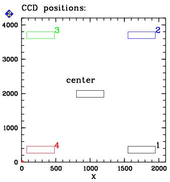
The contamination is measured in 5 different windows: 4 in the corners, and one central window. The central window defines the mean signal. The other windows are divided by that number and define the relative signal in that window. The contamination is defined as the relative signal in each of the 4 windows and plotted in report #3.

QC1_parameters

FITS key	QC1 database: table, name	definition	class*	HC_plot**	more docu
QC.CONTAM1	giraffe_ccd..conta1	contamination parameter in window1	HC
QC.CONTAM2	giraffe_ccd..conta2	contamination parameter in window2	HC
QC.CONTAM3	giraffe_ccd..conta3	contamination parameter in window3	HC
QC.CONTAM4	giraffe_ccd..conta4	contamination parameter in window4	HC
*Class: KPI - instrument performance; HC - instrument health; CAL - calibration quality; ENG - engineering parameter **There might be more than one, always check the link 'HC'.

Trending

A potential issue is contamination which is monitored in box 4. A set of four 400x200 pixels subwindows in the corners of the CCD is used to register the intensity there relative to a central reference subwindow. The fraction is trended over time here.

Monitoring contamination. Intensity in 4 subwindows relative to central window. Find here a sketch of the subwindows, same color coding as the data points.

History

Find a trending plot covering the full history of contamination here.

Typically, contamination builds up very slowly and then more strongly. Once the contamination parameter in one of the windows is below 0.9, an intervention is scheduled (heating of the CCD) to bring the CCD efficicency back to its nominal values.

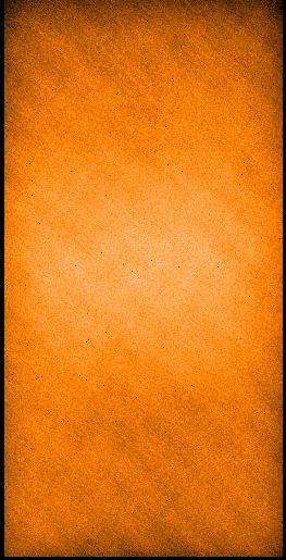
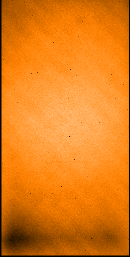
Below find a comparison between the image flats from 2003-04-28 and 2004-06-06 (just before an intervention). A contamination of about 7% has built up in window 4.

Monitoring contamination: Image flat from 2003-04-28 (no contamination).

Monitoring contamination: Image flat 2004-06-06 (strong contamination).

Scoring&thresholds Contamination

The relative contamination in quadrant #4 is scored. Based on the long-term behaviour, it fires an alert when its value is below 90%. This value is then used to trigger an operational action (decontamination).

Algorithm Contamination

- define 4 windows in the corners plus one in the centre
- measure mean signal in all five windows, divide by mean signal = signal in the central window #5
- the five windows are displayed in plot 2; the trended parameter is conta4.