Using PEARL to image Eta Vir
With the scan averaged data loaded from the previous step, issue
the following commands. Please note that throughout this exercise
you need some patience since the PEARL procedures use the Direct
Fourier Transform which is quite slow for the size of map we are
trying to work with!
set_complexvis
ComplexVis set.
pearl,'FKV0460',imsize=[180,300],cellsize=0.4
Warning(PEARL): imsize(0) must be odd, set to: 181
Warning(PEARL): imsize(1) must be odd, set to: 301
Mapsize is 72.4000 by 120.400
Computing dirty beam in 15 channels...
Computing dirty map..
Initial chisq= 24.980139
SVD: will edit 0 singular values!
Iteration 1 completed; chisq = 7.0768102
SVD: will edit 0 singular values!
Iteration 2 completed; chisq = 1.4564982
SVD: will edit 0 singular values!
Iteration 3 completed; chisq = 0.80119876
SVD: will edit 0 singular values!
Iteration 4 completed; chisq = 0.79117879
SVD: will edit 0 singular values!
Iteration 5 completed; chisq = 0.79115287
Final chisq= 0.79115287, reduced = 0.098894108
Iter= 6, Alamda= 0.000
SVD: will edit 0 singular values!
Synthesized beam 3.31332 by 2.01176 mas, pa = 158.324 degrees.
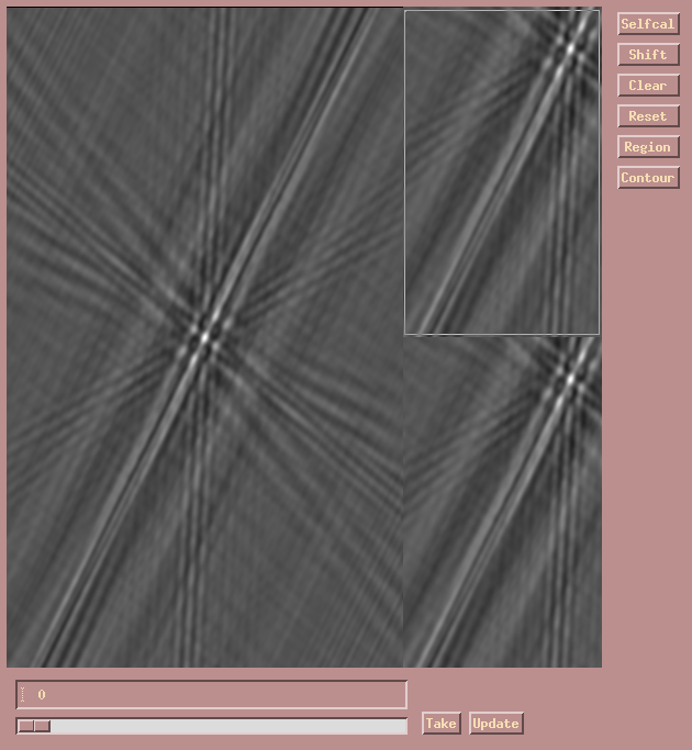
It will take a while (please be patient!) until a large widget is displayed
with areas containing the dirty beam, dirty map, and final map. (Click
on areas in the screen copy below for explanations of the buttons.)
First click the on the
Selfcal button,
then click the
Shift button
and enter these shift values (in mas): 25,45. After another delay, the
map will be shifted to the upper right so that we may image also the
tertiary component in the lower left (not yet visible!).
Now define a "Region"
(following the instructions as to how to set the
box in the smaller field in the upper right), and use 5000,4 for the
Teff,log(g) combination to use for model CLEAN components.
(This step is part of the here unused multi-wavelength capability of PEARL.)
Notice that the CLEAN slider is not active until the region is set.
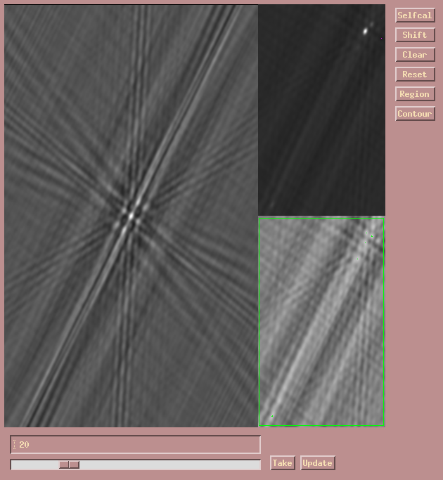
You should then be looking at
the following display.
This is the PEARL widget. It is a clickable map for explanations of the maps
and buttons.

To begin CLEANing the map click/drag on the CLEAN slider. Due to the
large size of the image there is again a delay in executing CLEAN, so wait
for the green CLEAN window (i.e. the Region) to show up in the lower right
residual map, along with the green colored CLEAN components. You can now
adjust the slider to the left and right to select the desired number of
CLEAN components. At this stage, it is important to subtract not too
many components since most of them would be associated with self-calibration
artefacts. Select about 30, as shown here.

Click Update to
add the selected number of CLEAN component to the
current model (which was empty at the start), self-calibrate the phases, subtract
the CLEAN components from the data, and re-display the updated residual and final
maps. The CLEAN slider moves back to zero for a new cycle of hybrid mapping. For the
next iteration, just subtract about 20 CLEAN components.

After this is complete, do two more "Update" iterations subtracting all 100
CLEAN components in each step. The maps should then look something like this.

Notice how the residual map rms, and printed to the message window, decreases.
At the same time, you can see how the residual map (in the lower right)
only shows noise and residual dirty beam patterns.
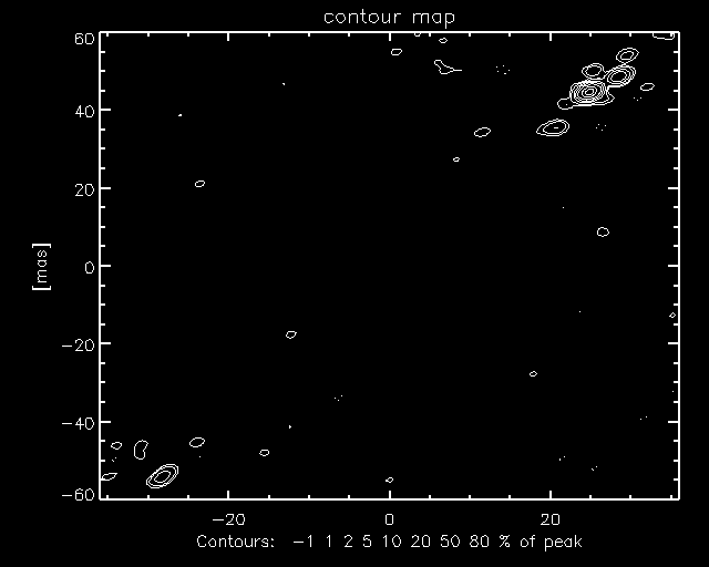
Now click on "Contour", and a map similar to the following should
be displayed.

Remember that you may not get the same result, and that the
quality of the maps varies. PEARL as implemented in OYSTER does not yet take
data weights into account, so there is room for improvement. If you want to see
how the map visibilities fit the observed visibilities, you have to read in
a special model file:
readmodel,image.model
calcmodel
This model file lists only one component (instead of the three in
etavir.model)
and uses the star_model.mode parameter to tell OYSTER that it is
a map stored with PEARL (rather than, e.g., a limb darkened disk) to transform.
You can then plot the observed and model data using the well known plot
widgets we have encountered earlier.
Next section
