Calibrating visibility amplitudes
Before calibrating the visibility data, we need to plot it and flag the blue
channels 21 to 32 because of their low signal-to-noise ratio. Select VisSq,
the uncalibrated raw (squared) visibility amplitude, and plot it versus
channel. Select all channels to be plotted, and to avoid getting a plot for each
of them separately, choose Option|All in 1. (Alternatively, the plot slice
can be set to 'ch'. For a data selection involving one or more indices with
a range of more than one element, e.g. all channels and all scans, the slice
parameter determines which index is NOT to be used as a loop index.)
The two figures show the visibility on the EW baseline before and after
editing.
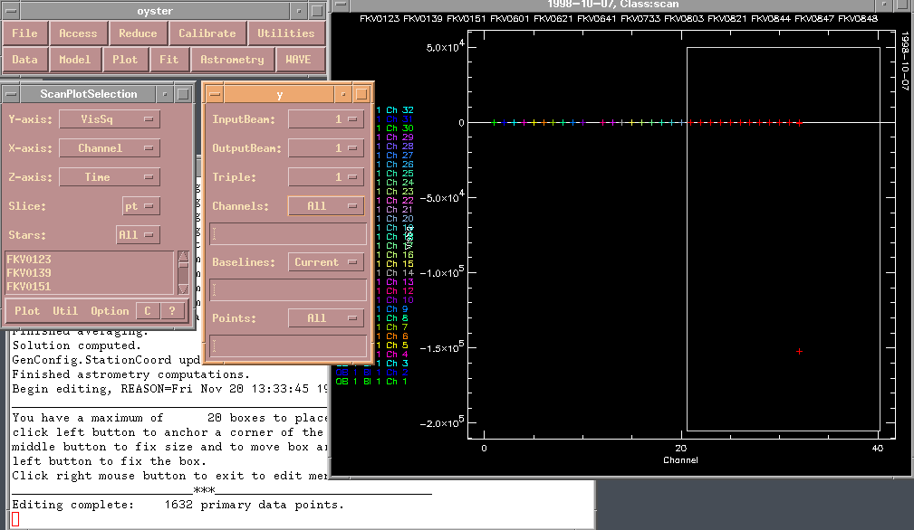
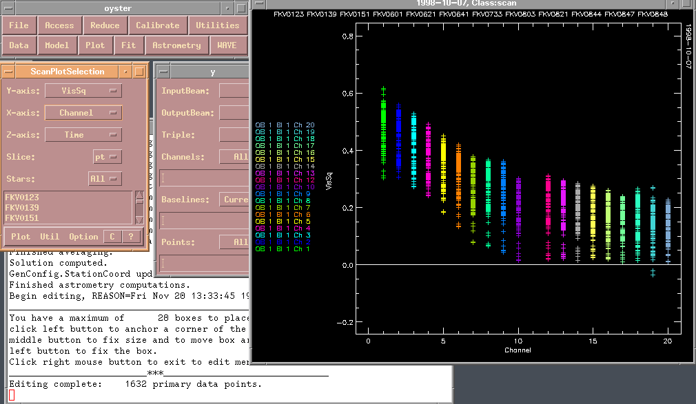 Note the way the y-axis is labeled, with each colored label corresponding to
a plot of the same color, all of them in the same frame. Also note that data
from channel 11 is absent, since the back ground data for this channel had
been flagged. The hierarchical editing scheme employed by OYSTER ensures that
data dependent on the type being flagged is also flagged. For example, if
count rates are flagged, visibilities for the same channel are unlikely to
be unaffected and have to be removed too. On the other hand, if visibility
amplitudes are flagged, the photon rate of the same channel is left unchanged
because the reasons leading to visibility corruption are not necessarily
related to detector performance.
A very simple but fairly decent way to calibrate visibilities of a program
star with a nearby unresolved calibrator (star) is to plot them side by side
versus time, smooth the calibrator visibility variations with time and apply
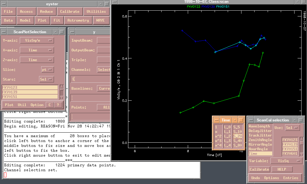
the resulting normalization factors to the program star. The following figure
shows two nearby calibrators and the program star (a binary, FKV0123). The
calibrators are well correlated, and based on the assumption that any
difference between them and the program star is due to actual difference
in the program star's structure, the calibration scheme is justified.

The calibration widget, Calibrate|Scans|CALIBRATE, allows you to select the
calibrators (here FKV0139, FKV0151), and to select the so-called indicators.
They are variables which have shown in the past, and not only for NPOI but
also for the Mark III interferometer, correlations with the visibility.
NOT ALL of those are applicable to a specific night! Usually it is just
one or two of them. But they are all listed because of our past experience
with other interferometers. Here we selected Time, and from a small widget
which is created for each indicator, a function to be used to model the
correlation. In this example, I chose S_20, which is a smoothing function
of 20 minutes length. The base function terms in the left column are polynomial
terms, in the middle column Legendre polynomials. These can be used
simultaneously with other indicators.
In the plot widget, we select the stars to which the calibration should be
applied. Do not forget to include the calibrators themselves in this selection!
The data selection defines which data is to be used to compute the correlation
parameters, with the exception that if the Option|Loop parameter is selected
in the calibration widget, the channels are calibrated independently, doing
every selected channel. As the variable to be calibrated, we selected VisSq
in the calibration widget. (The variable selected in the plot widget is
for plotting purposes only!)
It is actually VisSq c/e, initially set to VisSq/e, which is used for the
determination of the parameters. (By doing this we can stack several
calibrations on top of each other.) Click on Calibrate to compute the
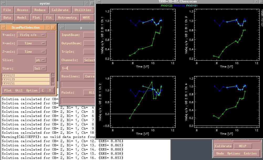
parameters and apply the results to the selected stars. The following figure
shows the results for 4 channels.

Note that the two calibrator star's visibilities are around unity, whereas the
binary star's amplitudes are significantly lower. Also look at the rms
information printed in the message window.
Next stop
Back to tour page
Back to main help page

 Note the way the y-axis is labeled, with each colored label corresponding to
a plot of the same color, all of them in the same frame. Also note that data
from channel 11 is absent, since the back ground data for this channel had
been flagged. The hierarchical editing scheme employed by OYSTER ensures that
data dependent on the type being flagged is also flagged. For example, if
count rates are flagged, visibilities for the same channel are unlikely to
be unaffected and have to be removed too. On the other hand, if visibility
amplitudes are flagged, the photon rate of the same channel is left unchanged
because the reasons leading to visibility corruption are not necessarily
related to detector performance.
