Quality Control and
Data Processing
UVES: ECH: System efficiency
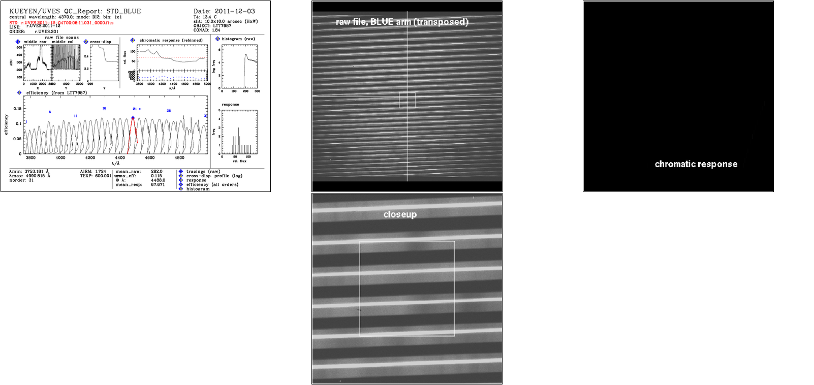
This tutorial provides information on the system efficiency. A monitoring is done frequently on STD_STAR data when conditions are CLEAR. Each STD_STAR OB makes a single observation of a spectrophotometric standard star in a specific instrument and wavelength setup, thus allowing evaluation of the instrument+telescope+atmosphere efficiency. In addition of a regular efficiency measurement, these STD provide a measurement of the spectral response. They are taken with the slit width set to 5 or 10 arcseconds. The flux standard table is included in the calSelector data sets. Standard stars are observed in three dichroic settings (346+580, 390+564, and 437+860, 1x1 binning), independently of the settings used for science observations during the night. These three dichroic settings are measured every night with science data. They are acquired close to twilight, with standards taken from a small set of stars with few spectral features. A second set of measurement is done once a month under Photometric conditions. These are used to measure the efficiency of the instrument.  Parameters trended
The montage displays: The efficiency table can be plotted, per order, over wavelength. The blaze wavelength of each order and the corresponding efficiency value there is written as QC1 parameter into the FITS header.
The max_effic parameter is used for trending, assuming that all efficiency curves per setting are similar apart from a scaling factor. Their trending with time primarily reflects efficiency variations of instrument components.
The proper selection of input data is crucial. Accepting all max_effic values as produced by the pipeline creates a large scatter. Reasons for this are: High-airmass data have the spectrum in the blue exposures shifted off-center which, especially in combination with a high sky level, brings the pipeline algorithm to assume an unrealistic background, with odd results for the efficiency. The same effect is observed under bad seeing since then the SKY level is unreliable as well. Stars with a rich absorption line spectrum tend to produce a larger scatter since max_effic is monochromatic. Scoring&thresholds Parameters trended The minimum threshold is set tighter than the higher threshold. False detections are made most often in the case of an observation in bad conditions.
The trending of the System Efficiency parameters during the life time of the instrument is best be seen with the full history trending plots shown here: FULL history. For the RED wavelength, the regular recoating of the mirror is illustrated by the jumps every 18 months. The pipeline processes the raw STD data (de-bias, flatten, average extraction), divides the flux table into the result and finally transforms into a fractional efficiency (where 0.1 means 10% of all incoming photons are registered on the CCD). The pipeline delivers an efficiency table (called UV_PEFC).
Response_fluxcalib
Response Curves and Flux Calibration The UVES pipeline produces response curves from STD calibration frames. Each exposure produces an individual response curve. Under ideal conditions (night is photometric, airmass is low, wide slit) each response curve provides a flux calibration for science data taken at the same setting and slit width. Realistically, the individual response curves are not always of ideal quality. A careful selection of these curves would yield master response curves of better quality. These curves are created for spcific settings and periods This set can be used for flux calibration of the reduced science data. With the upgrade of one of the red CCDs in 2009 it became obviously wrong to apply the old master reponse curves to the post-2009 UVES data.Unfortunately this was not immediately recognized on the QC side, and therefore the master response curves from 2004 were still applied for flux calibration until October 2011. Apart from the wrong usage of the response curve for the old red CCD, the application of the other two response curves for flux calibration was tolerable since the changes in the response curves are minor and slow. Historical response curves Major events that affected the shape and the level of the historical response curves: Note:
After the red CCD Upper Chip upgrade: the master responses for the 760 and 860 settings have been updated. The 860 curve for the new CCD is a scaled version of the one for the old CCD, the 760 curves are derived from the 860 ones. For the 580 and 564 it was found that the new CCD had no impact within the aimed accuracy. The master response curves are not updated due to manpower constraints. They are expected to slowly evolve with time but generally are good enough even for later epochs given the intrinsic innacuracies of the flux calibration. The user may prefer to create, from STD star measurements, selected individual response curves around the date of the science observations and apply them for flux calibration. See also the link below. top Flux calibration i To give an idea about the impact of the flux correction on the large-scale spectral slope, and about the precision that can be achieved, we have prepared a tutorial about flux calibration. Here you can also find a description of how to flux-calibrate your UVES data. tutorial on flux calibration tutorial on flux calibration
|
||||||||||||||||||||||||||||||||||||||||||||||||||||||||||||||||||||||||||||||||||||||||||||||||||||||||||||||||||||||||||||||||||||||||||||||||||||||||||||||||||||||||||||||
| |
||||||||||||||||||||||||||||||||||||||||||||||||||||||||||||||||||||||||||||||||||||||||||||||||||||||||||||||||||||||||||||||||||||||||||||||||||||||||||||||||||||||||||||||
 |
|
|||||||||||||||||||||||||||||||||||||||||||||||||||||||||||||||||||||||||||||||||||||||||||||||||||||||||||||||||||||||||||||||||||||||||||||||||||||||||||||||||||||||||||||