Arc recipe

For a given instrument setting, arcs consist of two or three exposures; one with the arc lamps off and additional exposures with one or both of the arc lamps on. The lamps are Xenon and Argon. The arcs are used to model the slit curvature and to derive the wavelength calibration. The eclipse recipe that analyses the arcs is called isaacp sw_arc. The input file(s) can either be a FITS file or an ASCII file containing a list of FITS files. If the input is a FITS file, one can select the line catalog. If the input is an ASCII file, then the value of specific keywords in the FITS headers are used to select the line catalog.

The recipe starts by classifying images based on instrument setting: a setting is defined by the resolution, the central wavelength and the slit.

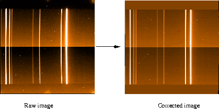
The slit curvature is modeled with a bivariate 2-d polynomial. If we let the distorted image be expressed in (u,v) coordinates, and the corrected image in (x,y) the curvature is modeled with:

u = a + bx + cy + dx² + ey² + fxy ; v = y

The dispersion relation (1st order) is computed by matching a xenon and/or argon atlas with the corrected spectra, which can be produced with the -c option. This is a weakness of the current version of the routine as a 3rd order fit provides a better description of the dispersion.

Users familiar with IRAF and/or MIDAS would notice that the correction for slit curvature and the wavelength calibration are done in two steps with this recipe, whereas using IRAF or MIDAS users can do it in one step.

The procedure produces two output files: a FITS table, which contains the fit to the slit curvature and the linear dispersion relation; and a PAF file, which contains the same information as the FITS file as well as additional quality control information.

The output FITS table is named [outname]_arc_setX_Y_Z.tfits where X is the setting number, Y the resolution (LR or MR), and Z the arc lamp (Xe, Ar, Xe+Ar), e.g. infile_arc_set2_MR_Xe+Ar.tfits. The corresponding PAF file would be called infile_arc_set2_MR_Xe+Ar.paf.

With the -c option, the recipe will produce the curvature corrected spectrum.

Figure  shows a raw image and the corresponding corrected one.

  

Figure: Slit curvature correction