Test results

Imaging
We have taken images through the pinhole masks for the SW broad band filters of the Hawaii (J,Js,H,Ks) and the Aladdin (J+Block,H,Ks) arms.

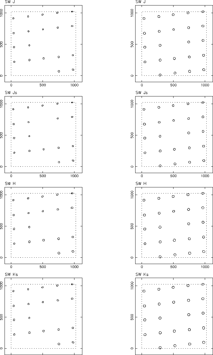
The pinhole mask images have been analysed using sextractor. For each pinhole image we measure the size of the major axis, the position angle of the major axis with the x-axis (measured counter clockwise), and the ratio of the axes (minor/major). The size of the major axis measured by sextractor is defined as the maximum spatial rms of the object profile along any direction. Table 1 gives the range of these measured quantities for each image. Table 2 gives links to the FITS files of these images. Figure 1 is a visualization of the sextractor results, showing the measured ellipses and their positions on the array. The size of the ellipses in this figure is exaggerated.

Table 1: Results of the SW & SWLW imaging tests with pinhole mask

pre-move			post-move
SW imaging tests with pinhole mask
filter	sigma	axis ratio	filter	sigma	axis ratio
J	$<$0.7	$>$0.7	J	$<$1	$>$0.8
Js	$<$0.7	$>$0.7	Js	$<$1	$>$0.8
H	$<$0.9	$>$0.7	H	$<$1.1	$>$0.8
Ks	$<$0.8	$>$0.7	Ks	$<$1.1	$>$0.9
SWLW imaging tests with pinhole mask
			J+Block	$<$1	$>$0.8
no data			H	$<$1.1	$>$0.8
			Ks	$<$1.1	$>$0.9

Table 2: FITS images of SW and SWLW pinhole mask tests

pre-move		post-move
SW imaging tests with pinhole mask
J	FITS image	J	FITS image
Js	FITS image	Js	FITS image
H	FITS image	H	FITS image
Ks	FITS image	Ks	FITS image
SWLW imaging tests with pinhole mask
		J+Block	FITS image
no data		H	FITS image
		Ks	FITS image

For these filters, the image quality with the current collimator position is acceptable. (We have also checked some of the narrow band filters, with the same result).

For the LW imaging (e.g. L & M band filters), the image quality in similar tests is very bad and we have to use the telescope to focus the image (which produces acceptable image quality).

Spectroscopy
For the pinhole mask + continuum spectra we have measured the gaussian fwhm of the spatial profile at 9 positions on the detector - at rows y $\approx$ 780, 320 and 80, and at x=200, 600 and 850 for collimator Position 1 and x=250, 500, 750 for collimator at Position 2. (The slightly different measurement positions for the different collimator positions are of no significance). The results are given in Table 3. If there is a significant spatial distortion it is noted as d (double peaked) or a (asymmetric) in the table. The plots of the spatial profiles at these positions in Figure 2 (SWS) and Figure 3 (LWS) give a better idea of the spatial distortion. Note that in the LWS hot pixels were not removed from the Position 1 data, and this causes additional spikes in a few of the profile plots (for 3.55 $\mu$m at x,y = (500,750) (750,750) (750,75) and for 4.75 $\mu$m at x,y = (500,75)).

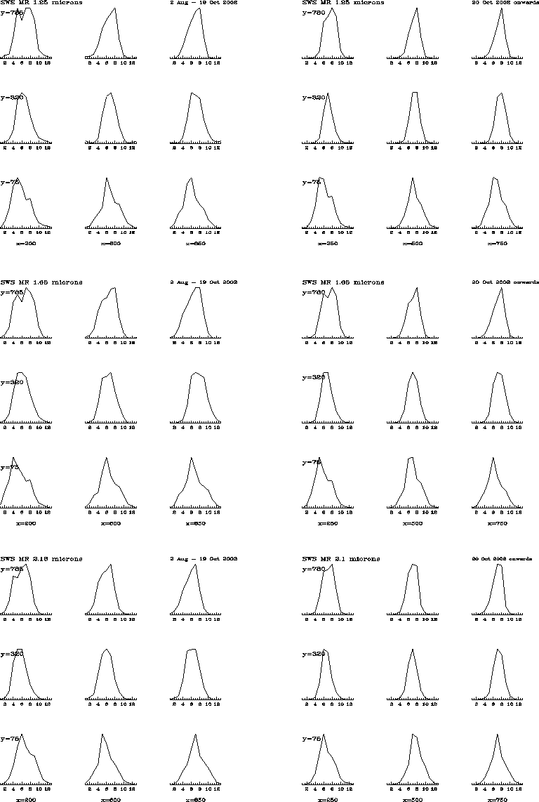
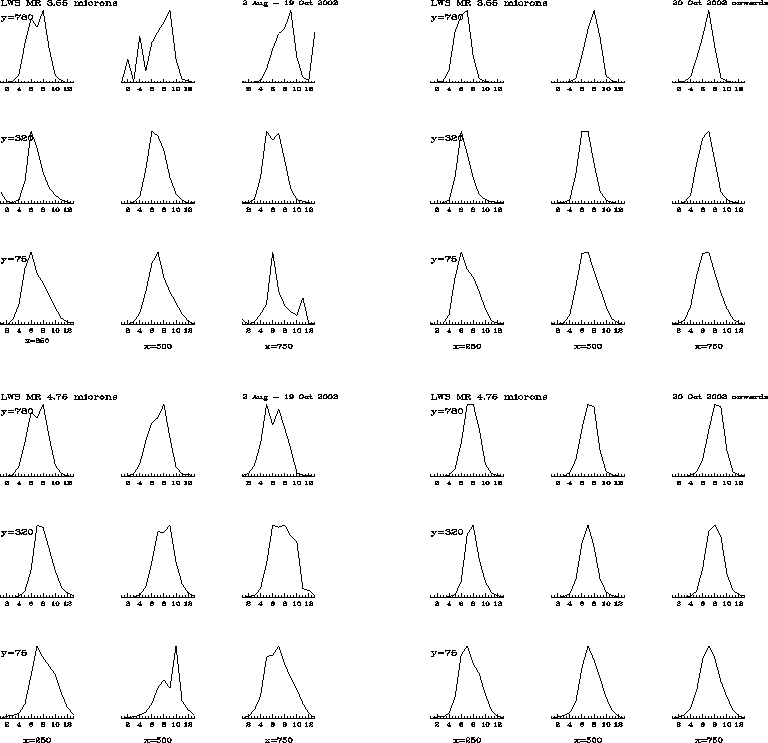
It is clear from the fwhm values and from the plots of the spatial profile that Position 2 (current position) produces better spectroscopic IQ than Position 1.

Table 3: Results of spectroscopy tests with pinhole mask and halogen lamp/thermal background. Measurements of the spatial fwhm at 9 positions on the image. `d' denotes a double-peaked profile and `a' denotes an asymmetric profile.

Position 1				Position 2
SWS MR 1.25 $\mu$m
	spatial fwhm				spatial fwhm
row	x=200	x=600	x=850	row	x=250	x=500	x=750
785	4.9d	3.8a	4.4a	780	3.5	2.7	2.7
320	3.5	3.5	4.0	320	2.4	2.6	2.8
80	5.4d	4.5a	5.3a	80	4.1	3.6	4.1
SWS MR 1.65 $\mu$m
row	x=200	x=600	x=850	row	x=250	x=500	x=750
785	5.4d	4.5d	5.0a	780	4.1	3.4	3.4
320	4.1	4.1d	4.6a	320	2.9	3.0	3.3
80	6.0a	4.9a	5.8	80	4.6	4.0	4.3
SWS MR 2.16 $\mu$m				SWS MR 2.10 $\mu$m
row	x=200	x=600	x=850	row	x=250	x=500	x=750
785	4.9d	4.1d	4.2a	780	4.2d	3.4a	3.1
320	3.5	3.5d	3.8a	320	2.9	3.0	3.3
70	4.3a	4.2a	4.6a	80	4.6d	4.0d	4.3d
LWS MR 3.55 $\mu$m
row	x=200	x=600	x=850	row	x=250	x=500	x=750
780	4.0d	3.7a	3.8a	780	3.0	2.8	2.7
315	2.6a	3.4a	3.8d	320	2.4	2.8	3.1
70	4.3a	4.2a	4.6a	80	4.1a	4.0	4.3
LWS MR 4.75 $\mu$m
row	x=200	x=600	x=850	row	x=250	x=500	x=750
780	4.0d	4.0a	4.2a	780	3.0	3.0	3.0
315	3.5a	4.0a	4.3	320	2.8	2.9	3.3
70	4.8a	4.8a	5.2	80	4.1a	3.8	4.2

Table 4: FITS images of spectroscopy tests with pinhole mask and halogen lamp/thermal background.

	Position 1	Position 2
SWS 1.25 $\mu$m	FITS image	FITS image
SWS 1.65 $\mu$m	FITS image	FITS image
SWS 2.16 $\mu$m	FITS image	FITS image
LWS 3.55 $\mu$m	FITS image$^{1}$	FITS image
LWS 4.75 $\mu$m	FITS image$^{1}$	FITS image
$^{1}$ - no dark subtracted

Sextractor was used to analyse the pinhole mask + arc lamp spectra. Again we measure the size and axis ratio of the pinhole images, and also the position angle (tilt) of each pinhole image. The position of the pinholes in the mask mean that we get 3 good spectra per image (from the central pinoles), at rows 780,320 and 80. In Table 5 we give the range of results per spectrum on the detector. The position angle is the angle between the major axis and the x-axis, measured counter clockwise (i.e. 90 degrees is aligned with the y-axis, that is, no tilt). In science data the absorption and emission lines will be tilted. This tilt should not be confused with the large scale tilt and curvature of the spectra, the tilt of the absorption/emission lines will remain after this large scale tilt has been removed.

Table 5: Results of spectroscopy tests with pinhole mask and arc lamps

pre-move				post-move
SWS MR 1.25 $\mu$m
row	sigma	axis ratio	tilt	row	sigma	axis ratio	tilt
780	$<$2	$>$0.6	50-60	780	$<$1.6	$>$0.6	40-60
320	$<$2	$>$0.6	45-60	320	$<$1.6	$>$0.6	40-60
80	$<$2.4	$>$0.6	60-70	80	$<$2	$>$0.5	60-75
SWS MR 1.65 $\mu$m
row	sigma	ellip	tilt	row	sigma	ellip	tilt
780	$<$2.4	$>$0.6	50-65	780	$<$1.8	$>$0.6	50-70
320	$<$2.3	$>$0.6	40-60	320	$<$1.8	$>$0.6	40-60
80	$<$2.8	$>$0.6	60-80	80	$<$2.2	$>$0.6	60-70
SWS MR 2.16 $\mu$m				SWS MR 2.10 $\mu$m
row	sigma	ellip	tilt	row	sigma	ellip	tilt
				780	$<$1.8	$>$0.6	50-70
no data				320	$<$1.6	$>$0.6	45-60
				80	$<$2	$>$0.6	60-70

Figure 1: Plots of SW imaging tests using pinhole mask. For each collimator position and filter we show the size and ellipticity of the images of the pinholes. The ellipse sizes have been exaggerated.

Figure 2: SW spectroscopy pinhole + halogen spatial profile plots.
The left hand column shows plots with collimator in Position 1 (2 Aug - 19 Oct 2002), the right hand column with collimator in Position 2 (20 Oct 2002 onwards). The spatial profile is plotted for 9 positions on the detector for each of three central wavelengths.

Figure 3: LW spectroscopy pinhole + halogen spatial profile plots.
The left hand column shows plots with collimator in Position 1 (2 Aug - 19 Oct 2002), the right hand column with collimator in Position 2 (20 Oct 2002 onwards). The spatial profile is plotted for 9 positions on the detector for each of two central wavelengths. Note that hot pixels were not removed from the position 1 data, and this causes additional spikes in a few of the profiles.