QC PLOTS
	CURRENT	HISTORY
RON
linearity
temperature
QC1 database (advanced users): browse | plot
Click on CURRENT to see the current trending (Health Check).    Click on HISTORY to see the historical evolution of the trending.

To calibrate the science data, there is no need in MIDI to measure bias exposure. The processing of the science data is done by substracting the two interferometric beams and the spectral channel for the same wavelength has a similar bias in both interferometric beams. To process the photmetric exposures, chopping is used and perform a systematic bias substraction.

One should take into account that the thermal background is the main contributor to the detector signal (compared to the photons from the observed object). The background is also removed by processing (as for the bias substraction of the interferometric beams or chopping) and the dynamic of the usefull signal is much smaller than the total dynamic of the detector.

The MIDI detector features a readout noise that affects the pixel levels. Though this noise is minimized by a very-low temperature cooling, shielding and tuning of the readout electronics, its value may affect the data quality of MIDI.

The readout noise of MIDI is monitored by taking a full-frame exposure with a large number of frames, with the MIDI shutter closed and with a minimum DIT (Detector Integration Time). The standard deviation of the pixel level over the frames is computed by the pipeline for each pixel, as well as the median of the standard deviation over all the pixels and all the frames.

A map of the standard deviation of the level for each pixel is produced, and the median (expressed in detector ADUs) of the level standard deviation over the whole detector area is given by the keyword: QC.DETRON.MEDIAN  

Pipeline steps:

QC1 parameters

Trending

History

The MIDI detector has been upgraded in November 2005, before the upgrade the conversion factor was of 145 e-/ADU. Since then the conversion factor is 90.

The RON is strongly dependant of the temperature of the detectors. The RON has been affected by several contamination of the detector due to power cuts. Below the results of two power cuts are shown: August 2007, when the detector went through a warmingup/backing cycle and Jan 2008. In September 2011 the detector was warmed and vacuum leaks were fixed..

MIDI RON: The example illustrate the increase in RON due to a power cut and a detector contamination

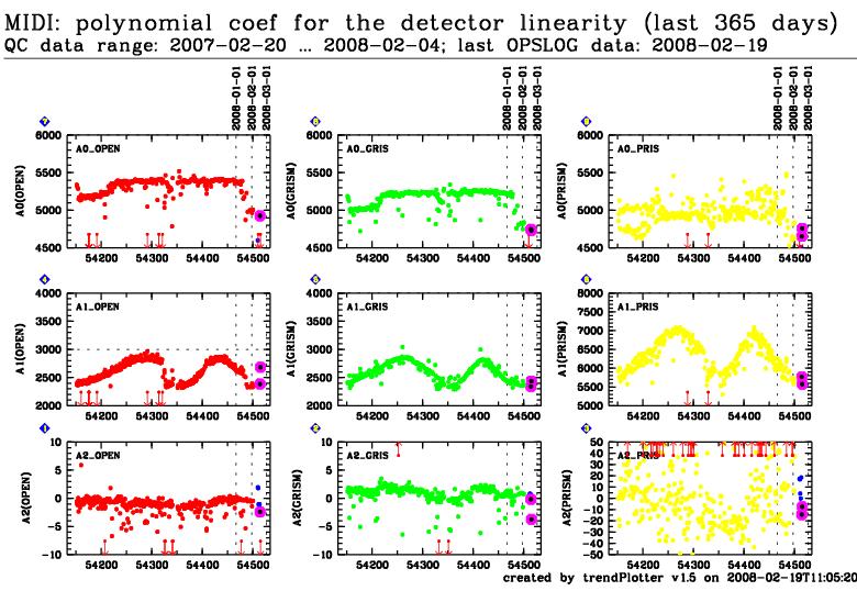
The linearity of the MIDI detector is an indicator if the quality of its response curve.

The detector linearity is measured with the following procedure:

- The MIDI detector is not designed for full frame imaging, so it is difficult to have all the pixels illuminated with a homogeneous level. The optical elements in the cryostat are moved to optimize the detector illumination. The detector is illuminated by the back-screen heated at a stable temperature.

- A set of N exposures is taken. If the frame exposure has an integration time T, the next one will be taken with T+ deltaT

- The pipeline calculate the coefficients of the polynomial fit of the average pixel value (over a windowed area) of the detector for 3 different configurations (image, prism and grism). The average level of the pixel in each exposure is used for the fit only if the level is bellow saturation (65535 ADUs).

The polynomial fit is: I(t) = A_0 + A_1 * t + A_2 * t^2 +A_3 * t^3, where I is the detector level in ADU and t the time in millisecond.  

The response curve should be as linear as possible, with A2 and A3 as close to zero as possible.

Because the pixels are not illuminated with the same flux, a large number of exposures are taken. Most of the pixels are already saturated in the last exposures (taken with the largest integration time). The integration time increment and the integration time of the first exposure are adjusted so the polynomial fit can be performed on the most illuminated pixels. The number of exposures has to be large enough. The integration time of the first exposure and the number of frames taken depends on the instrument setting:

• Imaging mode (QC1 database table midi_detlin, columns A0, A1, A2, A3, sigma for ins_disp = OPEN)
  
• Prism mode (QC1 database table midi_detlin, columns A0, A1, A2, A3, sigma for ins_disp = PRISM)
  
• Grism mode (QC1 database table midi_detlin, columns A0, A1, A2, A3, sigma for ins_disp = GRISM)
  

QC1 parameters

Trending

The coeffecients for the detector linearity are derived from a sequence of 12 images exposed between 2 and 24 ms for the OPEN mode, 1.2 and 9.6 ms for the PRISM mode and 2.4 and 24 ms for the GRISM mode.

Data are taken for the different dispersive elements (OPEN, PRISM and GRISM)

History

The linearity of the detector is strongly dependant of the temperature of the detectors. The following picture shows the trending recorded over 1 year, the 2 main power cut which affected MIDI are clearly visible.

As explained before, the RON and the linearity of the detector are strongly dependant of the temperature. It could be important to monitor the temperature of the different elements (beam combiner, camera ...)

QC1 parameters

• temperature of the camera (QC1 database table midi_detlin, column temp1_camera)
  
• temperature of the black screen (QC1 database table midi_detlin, column temp12_blackscreen)
  
• temperature of the filter wheel (QC1 database table midi_detlin, column temp2_filt_wheel)
  
• temperature of the dispersive elements (QC1 database table midi_detlin, column temp4_disp_elements)
  
• temperature of the beam combiner (QC1 database table midi_detlin, column temp5_beam_combiner)
  
• temperature of the mirror M1 (QC1 database table midi_detlin, column temp6_M1)
  
• temperature of the pinhole (QC1 database table midi_detlin, column temp7_pinhole)
  
• temperature of the shutter (QC1 database table midi_detlin, column temp8_shutter)
  
• temperature of the cryolite (QC1 database table midi_detlin, column temp10_cryolite)
  

Trending

At the beginning of operations, the temperature was trended for most of the different optical parts listed above. We now trend only the temperature and pressure of the camera.

History

Several parameters (RON, linearity of the detector) are dependant of the temperature of the detectors. Power cuts could cause an increase of the temperature and/or pressure.