


Next: Regularization in the wavelet
Up: Deconvolution
Previous: Deconvolution
Consider an image characterized by its intensity
distribution I(x,y), corresponding to the observation of an
object O(x,y) through an optical system. If the
imaging system is linear and shift-invariant, the relation between
the object and the image in the same coordinate frame is a
convolution:
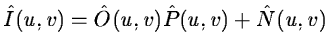
| I(x,y)= O(x,y) * P(x,y) + N(x,y) |
|
|
(14.99) |
P(x,y) is the point spread function (PSF) of the imaging system, and
N(x,y) is an additive noise. In Fourier space we have:
 |
|
|
(14.100) |
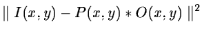
We want to determine O(x,y) knowing I(x,y) and P(x,y). This
inverse problem has led to a large amount of work, the main difficulties
being the existence of: (i) a cut-off frequency of the
PSF, and (ii) an intensity noise (see for example [6]).
Equation 14.99 is always an ill-posed problem.
This means that there is not a unique least-squares solution of minimal norm
 and a regularization is
necessary.
and a regularization is
necessary.
The best restoration algorithms are generally iterative [24].
Van Cittert [41] proposed the following iteration:
 |
|
|
(14.101) |
where  is a converging parameter generally taken as 1. In
this equation, the object distribution is modified by adding a term
proportional to the residual. But this algorithm diverges when we
have noise [12]. Another iterative algorithm is provided by
the minimization of the norm
is a converging parameter generally taken as 1. In
this equation, the object distribution is modified by adding a term
proportional to the residual. But this algorithm diverges when we
have noise [12]. Another iterative algorithm is provided by
the minimization of the norm
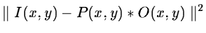 [21] and leads to:
![$\displaystyle O^{(n+1)} (x,y) = O^{(n)} (x,y) + \alpha P_s(x,y) * [I(x,y) - P(x,y) *
O^{(n)} (x,y)]$](img835.gif) |
|
|
(14.102) |
where
Ps(x,y)=P(-x,-y).
Tikhonov's regularization [40] consists of minimizing the term:
 |
|
|
(14.103) |
where H corresponds to a high-pass filter.
This criterion contains two terms;
the first one,
 ,
expresses
fidelity to the data I(x,y) and the second one,
,
expresses
fidelity to the data I(x,y) and the second one,
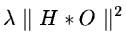 ,
smoothness of the restored image.
,
smoothness of the restored image.  is the
regularization parameter and represents the trade-off between
fidelity to the data and the restored image smoothness. Finding
the optimal value
is the
regularization parameter and represents the trade-off between
fidelity to the data and the restored image smoothness. Finding
the optimal value  necessitates use of numeric techniques such as
Cross-Validation [15] [14].
necessitates use of numeric techniques such as
Cross-Validation [15] [14].
This method works well, but it is relatively long
and produces smoothed images. This second point can be a real problem
when we seek compact structures as is the case in astronomical imaging.
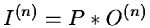
An iterative approach for computing maximum likelihood estimates may be used.
The Lucy method [#lucy<#15258,#katsaggelos<#15259,#adorf<#15260] uses such
an iterative approach:
![$\displaystyle O^{(n+1)} = O^{(n)} [ \frac{I}{I^{(n)}} \ast P^* ]$](img841.gif) |
|
|
(14.104) |
and
 |
|
|
(14.105) |
where P* is the conjugate of the PSF.
Next: Regularization in the wavelet
Up: Deconvolution
Previous: Deconvolution
http://www.eso.org/midas/midas-support.html
1999-06-15