Next: Regularization from significant structures
Up: Deconvolution
Previous: Regularization in the wavelet
Tikhonov's regularization and multiresolution analysis
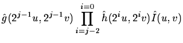
If wj(I) are the wavelet coefficients of
the image I at the scale j, we have:
where
wj(P) are the wavelet coefficients of the PSF at the scale j.
The wavelet coefficients of the image I are the product of convolution
of object O by the wavelet coefficients of the PSF.
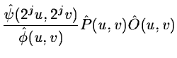
To deconvolve the image, we have to minimize for each scale j:
 |
|
|
(14.107) |
and for the plane at the lower resolution:
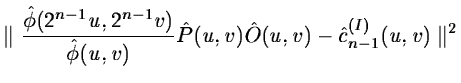 |
|
|
(14.108) |
n being the number of planes of the wavelet transform ((n-1) wavelet
coefficient planes and one plane for the image at the lower resolution).
The problem has not generally a unique solution, and we need to do
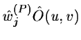
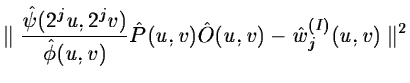
a regularization [40]. At each scale, we add the term:
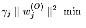 |
|
|
(14.109) |
This is a smoothness constraint. We want to have the minimum information
in the restored object. From equations 14.107, 14.108,
14.109, we find:
 |
|
|
(14.110) |
with:
and:
if the equation is well constrained, the object can be computed by a
simple division of  by
by  .
An iterative algorithm
can be used to do this inversion if we want to add other constraints such as
positivity. We have in fact a multiresolution Tikhonov's regularization.
This method has the advantage to furnish a solution quickly, but
optimal regularization parameters
.
An iterative algorithm
can be used to do this inversion if we want to add other constraints such as
positivity. We have in fact a multiresolution Tikhonov's regularization.
This method has the advantage to furnish a solution quickly, but
optimal regularization parameters  cannot be found directly,
and several tests are generally necessary before finding an acceptable
solution. Hovewer, the method can be interesting if we need to deconvolve
a big number of images with the same noise characteristics. In this case,
parameters have to be determined only the first time. In a general way,
we prefer to use one of the following iterative algorithms.
cannot be found directly,
and several tests are generally necessary before finding an acceptable
solution. Hovewer, the method can be interesting if we need to deconvolve
a big number of images with the same noise characteristics. In this case,
parameters have to be determined only the first time. In a general way,
we prefer to use one of the following iterative algorithms.
Next: Regularization from significant structures
Up: Deconvolution
Previous: Regularization in the wavelet
Petra Nass
1999-06-15

![\begin{eqnarray*}\hat N(u,v) = \hat\phi(u, v) [ \sum_j \hat P^*(u,v)\hat\psi^*(2...
... \hat P^*(u,v) \hat\phi^*(2^{n-1}u,2^{n-1}v) \hat c_{n-1}^{(I)}]
\end{eqnarray*}](img852.gif)