The data taken on sky are taken simultaneously with the 2 detectors using different dispersions (low, medium and high). The data in the 2 bands creates 2 different ABs (reduction blocks) and are processed by the pipeline using different pipeline parameters.
MATISSE instrument has different limiting magnitude in the 2 bands, so in some cases while the object is bright enough in one band, its flux is too faint in the other band resulting in a product in this band which is only "noise".
Some additional QC parameters are calculated by the QC script to identify if the product is valid (object within the instrument limiting magnitude) or not. They are valid_flag_target, valid_flag_flux, valid_flag_VisSNR and valid_flag_fluxSNR.
From these flags value, a global valid_flag is coded. For QC purposes, only valid_flag <=2 means that the pipeline product can be considered and looked at. For all the other combinations (for ex. Flux NOK) the valid_flag is set to 88.
Flux
Magnitude
SNR on Vis
SNR on flux
valid_flag
(from Vis or corr_flux)
(OK: flux > 0 for all the beams)
(OK: within the limiting mag for the setup)
(OK: SNR >2)
(OK: all the beams with flux>0 and SNRflux >2)
OK
OK
OK
OK
0
Corr_flux
OK
OK
OK
0
unknown
OK
OK
OK
0
OK
unknown
OK
OK
0
Corr_flux
unknown
OK
OK
0
unknown
unknown
OK
OK
0
OK
NOK
OK
OK
1
Corr_flux
NOK
OK
OK
1
OK
OK
only one SNR OK
only one SNR OK
2
Corr_flux
OK
only one SNR OK
only one SNR OK
2
unknown
OK
only one SNR OK
only one SNR OK
2
OK
unknown
only one SNR OK
only one SNR OK
2
The data taken on sky with DPR.CATG SCIENCE or CALIB are processed with the same recipe. Depending of the category, additional products can be calculated.
The input raw data consist in several files : files containing fringes (or photometry frames) and measurement on sky. The detector calibrations BADPIX, NONLINEARITY as well as the Observing flatfield (OBS_FLATFIELD) , the distortion map (SHIFT MAP), the Kappa matrix (KAPPA_MATRIX) are also needed or optional in certain cases (KAPPA_MATRIX).
The recipe mat_raw_estimates calls all data reduction steps which transform the measured raw frames to the average raw interferometric products like raw squared visibilities, raw closure phases and raw differential phases. The same recipe is applied to target or calibrator frames as well as to the fringe day time calibration.
The main recipe is divided in different reduction steps:
The input data (fringe and photometric beams) needs to be cleaned of detector and instrumental effects. This is done with the sub recipe mat_cal_image:
--Applying cosmetics on the input data (compensation of offset effects such as pixel bias, detector channel bias and cross talk)
--compensating for non linearity
--applying the flat field map to compensate for space-variant gain
--interpolating bad detector pixels
--applying the distorsion matrix to transform the coordinates of the data
mat_ext_beams: after the compensation for cosmetics, non linearity, distorsion, the recipe mat_ext_beams will:
--adjust the photometric contribution in the interferometric beams by applying the kappa matrix, shift and zoom
--remove the thermal background by substracting the average sky (measured via chopping) from the photometric beam intensity to get the photometric intensity produced by the target alone.
The result of these 2 recipes is a clean fringe pattern and clean phtometric estimates.
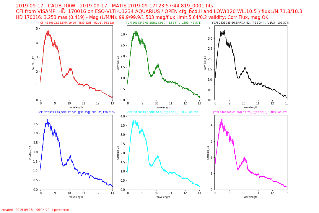
The raw correlated fluxes are calculated using mat_est_corr:
It derives the uncontaminated complex correlated flux from each recorded interferogram. The uncontaminated complex correlated flux is the Fourier Transform of the interferogram without its huge low frequency part which contaminates the fringes peaks. This contamination could be compensated by two methods :
applying the OPD modulation algorithm
by substraction of the photometric beams if they have been measured
The Optical Path Difference (OPD) is estimated using mat_est_opd:
This sub recipe estimates the OPD and the water vapor offset for each baseline and for each frame. It takes as input the correlated flux.
It allows also to estimate chromatic OPD by fitting the Matthar's model (2007). If ChromaticOpdFit=TRUE,
the output contains temperature and relative humidity offsets (Matthar's model).
The squared visibilities, the closure phases and the differential phase are computed using either coherent or incoherent processing:
--mat_proc_incoherent: calculates the average power and bi spectrum from all selected frames.
From these aver:ages, the photometrically calibrated square raw visibility and the raw closure phase are derived for each spectral channel.
In the low resolution mode, teh coherence length and the amplitude of teh atmospheric OPD varisations are similar, so the fringe contrast depends on the actual atmospheric OPD. This OPD has been calculated previously (mat_est_opd) and is used to compensare the fringe contrast loss
As a by-product, this recipe computes the spectrum of the target.
--mat_proc_coherent
This plugin runs the coherent processing. It computes the raw differential phase and the raw correlated flux (or visibility).
The last step is to merge the intermediate results calculated by the sub-recipes and create a final product which is OIFITS compliant.
This is done with the sub-recipe mat_merge_results
There is one product per BCD configuration: OUT-OUT, IN-IN, OUT-IN, IN-OUT.
If the object observe is a calibrator (DPR.CATG=CALIB), an additional recipe is run to estimate the Transfer Function which will be applied to calibrate the science target.
The plugin is mat_est_tf:
It is run before the merging of the intermediate products and the result will be merged in the OIFITS.
It estimates the Transfer Function from one or several
RAW_VIS2 files corresponding to observations of calibrator stars.
To calculate the TF, the angular diameter (and its error) of the calibator should be known. These are retrieved from catalog provided in the sof
.The recipes creates a RAW_TF2 FITS file containing the
transfer function for each RAW_VIS2 file given as input.
The QC parameters describing the visibilities (or correlated fluxes), the SNR on the visibilities, and the Transfer function (if avalaible) are trended for both detectors and the different resolution.
The visibilities are shown in the trending plots.
The SNR on the visibilities are shown in the trending plots If the correlated fluxes are calculated, these are shown in the trending plots.
None of the QC parameters described above are scored in the HC plots.
Thresholds for the scoring of the parameters are based on "experience". The TF should be between 0.25 and 1 and the SNR should not be smaller than 2.
The measured Visibility on the target is always lower than the expected theoritical visibility. Instrumental imperfections coupled with the atmospheric turbulence contribute to decrease the coherency of the light recorded from the telescopes.
We calculate the instrumental TF as TF=measured Vis/theoritical Vis.
To determine the value TF, a calibrator (unresolved star or with a known diameter) is observed. The theoritical Vis is calculated using the diameter which is in the calibrator catalog (input to the recipe).
Given the very wide band nature of MATISSE (3 to 13 microns), teher are very few or even no calibration star optimal for both LM and N bands. Very often the TF calculated in one of teh band (most often band N) is just noise.
In operations often 2 different calibrators are observed to calibrate the two bands of the same scientific target.
None of the QC parameters described above are scored in the HC plots.
Thresholds for the scoring of the parameters are based on "experience". The TF should be between 0.25 and 1 and the SNR should not be smaller than 2.
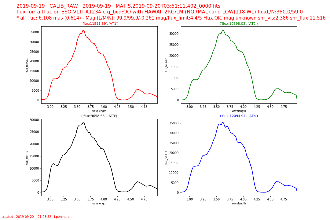
Depending of the raw data taken, the recipe mat_raw_estimates also estimate the spectrum of the object for the four different beams (telescopes). The ratio of the fluxes are calculated as QC parameters
The flux ratio between the different beams and the total flux is scored and should be between .15 and .35. Ideally, the total flux should be divided equally between the 4 telescopes .
 Visibility