[Top] [Prev] [Next] [Bottom]

3.5 Analyzing HST Spectra

This section describes some IRAF/STSDAS tasks that can be used for analyzing and manipulating spectral data. Certain of these tasks operate directly on HST data files created by the pipeline. However, a number of the most useful IRAF tasks, such as splot, require special preparations of data other than STIS two-dimensional spectra. Before discussing these tasks we will first show how to recast your data into forms that are more generally accessible.

3.5.1 Preparing FOS and GHRS Data

The FOS and GHRS data reduction pipelines store fluxes and wavelengths in separate files. In GEIS format, the .c1h file contains the flux information and the .c0h file contains the wavelength information. Because IRAF tasks generally require both the flux and wavelength information to reside in the same file, you will probably want to create a new file that combines these quantities.

Several options for combining flux and wavelength information are available:

resample: This simple task resamples your flux data onto a linear wavelength scale, creating a new flux file containing the starting wavelength of the new grid in the CRVAL1 keyword and the wavelength increment per pixel in the CD1_1 keyword. Encoding the wavelength information into these standard FITS header keywords makes this format quite portable, but the resampling process loses some of the original flux information. In addition, the error (.c2h) and data quality (.cqh) files cannot be similarly resampled, limiting the usefulness of this technique.
mkmultispec: This task writes wavelength information into the header of a flux file while preserving all the original information. It is therefore a better choice than resample for most applications, and we describe it in more detail below.
imtab: An alternative to writing wavelength information into the header is to use the imtab task to create a table recording the wavelength, flux, and if desired, the error data corresponding to each pixel. Many STSDAS tasks, such as those in the STSDAS fitting package, can access data in tabular form, so we describe this approach in more detail as well.

mkmultispec

The most convenient method of combining wavelength and flux information, and one that has no effect on the flux data at all, is to use the mkmultispec task. This task places wavelength information into the headers of your flux files according to the IRAF multispec-format World Coordinate System (WCS). The multispec coordinate system is intended to be used with spectra having nonlinear dispersions or with images containing multiple spectra, and the format is recognized by many tasks in IRAF V2.10 or later. For a detailed discussion of the multispec WCS, type help specwcs at the IRAF prompt.

The mkmultispec task can put wavelength information into the flux header files in two different ways. The first involves reading the wavelength data from the .c0h file, fitting the wavelength array with a polynomial function, and then storing the derived function coefficients in the flux header file (.c1h) in multispec format. Legendre, Chebyshev, or cubic spline (spline3) fitting functions of fourth order or larger produce essentially identical results, all having rms residuals less than 10-4 Å, much smaller than the uncertainty of the original wavelength information. Because these fits are so accurate, it is usually unnecessary to run the task in interactive mode to examine them.

If there are discontinuities in the wavelengths, which could arise due to the -splicing of different gratings, you should run mkmultispec in interactive mode to verify the fits.

Because mkmultispec can fit only simple types of polynomial functions to wavelength data, this method will not work well with FOS prism data, because of the different functional form of the prism-mode dispersion solution. For prism spectra, use the header table mode of mkmultispec (see below) or create an STSDAS table using imtab.

The other method by which mkmultispec can incorporate wavelength information into a flux file is simply to read the wavelength data from the .c0h file and place the entire data array directly into the header of the flux (.c1h) file. This method simply dumps the wavelength value associated with each pixel in the spectrum into the flux header and is selected by setting the parameter function=table. To minimize header size, set the parameter format to a suitable value. For example, using format=%8.7g will retain the original seven digits of precision of the wavelength values, while not consuming too much space in the flux header file.

Be aware that there is a physical limit to the number of header lines that can be used to store the wavelength array (approximately 1000 lines). This limit cannot be overridden. Under ordinary circumstances this limitation is not an issue. However, if many spectral orders have been spliced together, it may not be possible to store the actual wavelength array in the header, and a fit must be done instead.

imtab

Another way to combine wavelengths with fluxes is to create an STSDAS table from your spectrum. The imtab task in the STSDAS ttools package reads a GEIS format spectral image and writes the list of data values to a column of an STSDAS table, creating a new output table if necessary. The following example shows how to create a flux, wavelength, and error table from group eight of a GEIS-format FOS dataset:

cl> imtab y0cy0108t.c0h[8] y0cy0108t.tab wavelength

cl> imtab y0cy0108t.c1h[8] y0cy0108t.tab flux

cl> imtab y0cy0108t.c2h[8] y0cy0108t.tab error

The last word on each command line labels the three columns "wavelength", "flux", and "error".

Constructing tables is a necessary skill if you plan to use certain tasks-such as those in the STSDAS fitting package-that do not currently recognize the multispec format WCS header information. Tabulating your spectra is also the best option if you want to join two or more spectra taken with different gratings into a single spectrum covering the complete wavelength range. Because the data are stored as individual wavelength-flux pairs, you do not need to resample, and therefore degrade, the individual spectra to a common, linear dispersion scale before joining them. Instead, you could create separate tables for the spectra from different gratings, and then combine the two tables using, for example, the tmerge task:

cl> tmerge n5548_h13.tab,n5548_h19.tab n5548.tab append

Note that you will first have to edit out any regions of overlapping wavelength from one or the other of the input tables so that the output table will be monotonically increasing (or decreasing) in wavelength.

3.5.2 Preparing STIS Spectra for Analysis

Calibrated STIS spectra emerge from the pipeline either as two-dimensional images (_x2d files) or as one-dimensional spectra in tabular form (_x1d files.) You can analyze calibrated two-dimensional STIS spectra in IRAF as you would any other long-slit spectral image, because their headers already contain the necessary wavelength information. Tabulated STIS spectra can be analyzed directly using STSDAS tasks that understand the selectors syntax described on page 2-9. However, to use IRAF tasks, such as splot, that rely on the multispec WCS or to use STSDAS tasks that do not understand three-dimensional tables, you will have to prepare your data appropriately. This section describes two useful tasks for putting your data in the proper form:

tomultispec: This task is the STIS analog to mkmultispec, described above; it extracts STIS spectra from tables and writes them as IRAF spectral images with wavelength information in the header.
txtable: This task extracts specified data arrays from STIS table cells and places them in conventional two-dimensional tables for easier access.
tximage: Extracts specified data arrays from STIS table cells and places them into 1-D images. This task can write single group GEIS files.

tomultispec

The tomultispec task in the stsdas.hst_calib.ctools package extracts one or more spectral orders from a STIS table, fits a polynomial dispersion solution to each wavelength array, and stores the spectra in an output file in original IRAF format (OIF), using the multispec WCS. This task is layered upon the mkmultispec task, which performs a similar operation for FOS and GHRS calibrated spectra (see page 3-21). Most of the parameters for tomultispec echo those for mkmultispec. As a helpful navigational aid, the STIS spectral order numbers are written to the corresponding beam numbers in the multispec image; the aperture numbers are indexed sequentially starting from one. You can choose to fit the dispersion solution interactively, but the default fourth-order Chebyshev polynomial will likely suffice for all STIS spectral orders, except for prism-dispersed spectra. However, you cannot use the interactive option if you are selecting more than one order from the input file.

For example, if you want to write all spectral orders from the STIS file myfile_x1d.fits to a multispec file, you can type:

	cl> tomultispec myfile_x1d.fits new_ms.imh

Note that the .imh suffix on the output file specifies that the output file is to be an OIF file. This format is similar to GEIS format, in that it consists of two files: a header file (.imh) and a binary data file (.pix). The output format for tomultispec will always be OIF.

If you want to select particular spectral orders, rather than writing all the orders to the multispec file, you will need to use the selectors syntax. To select only the spectrum stored in row nine of the input table, the previous example would change to:

cl> tomultispec "myfile_x1d.fits[r:row=9]" new_ms.imh

Note that the double quote marks around the file name and row selector are necessary to avoid syntax errors. To select a range of rows, say rows nine through eleven, you would type:

cl> tomultispec "myfile_x1d.fits[r:row=(9:11)]" new_ms.imh

You can also select rows based upon values in some other column. For example, to select all rows whose spectral order lies in the range 270 to 272, type:

cl> tomultispec "myfile_x1d.fits[r:sporder=(270:272)]" \

>>> new_ms.imh

The calibrated flux is extracted by default. However, other intensity data can be specified by setting the flux_col parameter.

Be careful not to restrict the search for matching rows too heavily.

Column selectors cannot be used with tomultispec.

Choose the type of fitting function for the tomultispec dispersion solution with care. Using the table option, which writes the entire wavelength array to the image header for each order, will fail if more than about three orders are selected. This restriction results from a limit to the number of keywords that can be used to store the dispersion relation.

txtable

Tabulated STIS spectra are stored as data arrays within individual cells of FITS binary tables (see Chapter 2, page 2-9). These tables are effectively three-dimensional, with each column holding a particular type of quantity (e.g., wavelengths, fluxes), each row holding a different spectral order, and each cell holding a one-dimensional array of values spanning the wavelength space of the order. The txtable in the tables.ttools package extracts these data arrays from the cells specified with the selectors syntax and stores them in the columns of conventional two-dimensional binary tables.

For example, suppose the first extension of the FITS file data.fits contains a STIS echelle spectrum and you want to extract only the wavelength and flux arrays corresponding to spectral order 68. You could then type:

tt> txtable "data.fits[1][c:WAVELENGTH,FLUX][r:sporder=68]" \

>>> out_table

This command would write the wavelength and flux arrays to the columns of the output table out_table. To specify multiple rows in a tabulated echelle spectrum, you would type:

tt> txtable "data.fits[1][c:WAVELENGTH,FLUX][r:row=(10:12)]" \

>>> echl

This command would generate three separate output files named echl_r0010.tab, echl_r0011.tab, and echl_r0012.tab.

See the online help for more details on txtable and the selectors syntax, and remember to include the double quotation marks.

tt> tximage "data.fits[1][c:WAVELENGTH][r:row=4]" wave.hhh

tt> tximage "data.fits[1][c:FLUX][r:row=4]" flux.hhh

3.5.3 General Tasks for Spectra

IRAF has many tasks for analyzing both one- and two-dimensional spectral data. Many observers will already be familiar with noao.onedspec and noao.twodspec packages, and those who are not should consult the online help. Table 3.5 lists some of the more commonly used IRAF/STSDAS spectral analysis tasks, and below we briefly describe splot, one of the most versatile and useful. Remember that many of these tasks expect to find WCS wavelength information in the header, so you should first run mkmultispec or tomultispec on your data, if necessary.

**Tasks for Working with Spectra**
Task	Package	Input Format	Purpose
boxcar	images.imfilter	Image	Boxcar smooth a list of images
bplot	noao.onedspec	Multispec image	Plot spectra non-interactively
continuum	noao.onedspec	Image	Continuum normalize spectra
fitprofs	noao.onedspec	Image	Non-interactive Gaussian profile fitting to features in spectra and image lines
gcopy	stsdas.toolbox.imgtools	GEIS image	Copy multigroup images
grlist	stsdas.graphics.stplot	GEIS image	List file names for all groups in a GEIS image; used to make lists for tasks that do not use group syntax
grplot	stsdas.graphics.stplot	GEIS image	Plot arbitrary lines from 1-D image; overplots multiple GEIS groups; no error or wavelength information is used
grspec	stsdas.graphics.stplot	Multispec GEIS image	Plot arbitrary lines from 1-D image; stack GEIS groups
magnify	images.imgeom	Image	Interpolate spectrum on finer (or coarser) pixel scale
nfit1d	stsdas.analysis.fitting	Image, table	Interactive 1-D non-linear curve fitting (see page 3-29)
ngaussfit	stsdas.analysis.fitting	Image, table	Interactive 1-D multiple Gaussian fitting (see page 3-29)
poffsets	stsdas.hst_calib.ctools	GEIS image	Determine pixel offsets between shifted spectra
rapidlook	stsdas.hst_calib.ctools	GEIS image	Create and display a 2-D image of stacked 1-D images
rcombine	stsdas.hst_calib.ctools	GEIS image	Combine (sum or average) GEIS groups in a 1-D image with option of propagating errors and data quality values
resample	stsdas.hst_calib.ctools	GEIS image	Resample FOS and GHRS data to a linear wavelength scale (see page 3-21)
sarith	noao.onedspec	Multispec image	Spectrum arithmetic
scombine	noao.onedspec	Multispec image	Combine spectra
sfit	noao.onedspec	Multispec image	Fit spectra with polynomial function
sgraph	stsdas.graphics.stplot	Image, table	Plot spectra and image lines; allows overplotting of error bars and access to wavelength array (see page 3-17)
specalign	stsdas.hst_calib.ctools	GEIS image	Align and combine shifted spectra (see poffsets)
specplot	noao.onedspec	Multispec image	Stack and plot multiple spectra
splot	noao.onedspec	Multispec image	Plot and analyze spectra & image lines (see page 3-27)

splot

The splot task in the IRAF noao.onedspec package is a good general analysis tool that can be used to examine, smooth, fit, and perform simple arithmetic operations on spectra. Because it looks in the header for WCS wavelength information, your file must be suitably prepared. Like all IRAF tasks, splot can work on only one group at a time from a multigroup GEIS file. You can specify which GEIS group you want to operate on by using the square bracket notation, for example:

cl> splot y0cy0108t.c1h[8]

If you don't specify a group in brackets, splot will assume you want the first group. In order to use splot to analyze your FOS or GHRS spectrum, you will first need to write the wavelength information from your .c0h file to the header of your .c1h files in WCS, using the mkmultispec task (see page 3-21).

The splot task is complex with many available options described in detail in the online help. Table 3.6 summarizes a few of the more useful cursor commands for quick reference. When you are using splot, a log file saves results produced by the equivalent width or de-blending functions. To specify a file name for this log file, you can set the save_file parameter by typing, for example:

cl> splot y0cy0108t.c1h[8] save_file=results.log

If you have used tomultispec to transform a STIS echelle spectrum into .imh/.pix OIF files with WCS wavelength information (see page 3-23), you can step through the spectral orders stored in image lines using the ")", "(", and "#" keys. To start with the first entry in your OIF file, type:

cl> splot new_ms.imh 1

You can then switch to any order for analysis using the ")" key to increment the line number, the "(" key to decrement, and the "#" key to switch to a specified image line. Note the beam label that gives the spectral order cannot be used for navigation. See the online help for details.

**Useful splot Cursor Commands**
Command	Purpose
Manipulating spectra
f	Arithmetic mode; add and subtract spectra
l	Convert spectrum from fto f(invert transformation with "n")
n	Convert spectrum from fto f
s	Smooth with a boxcar
u	Define linear wavelength scale using two cursor markings
Fitting spectra
d	Mark two continuum points & de-blend multiple Gaussian line profiles
e	Measure equivalent width by marking points around target line
h	Measure equivalent width assuming Gaussian profile
k	Mark two continuum points and fit a single Gaussian line profile
m	Compute the mean, RMS, and S/N over marked region
t	Enter interactive curve fit function (usually used for continuum fitting)
Displaying and redrawing spectra
a	Expand and autoscale data range between cursor positions
b	Set plot base level to zero
c	Clear all windowing and redraw full current spectrum
r	Redraw spectrum with current windowing
w	Window the graph
x	Etch-a-sketch mode; connects two cursor positions
y	Overplot standard star values from calibration file
z	Zoom graph by a factor of two in X direction
$	Switch between physical pixel coordinates and world coordinates
General file manipulation commands
?	Display help
g	Get another spectrum
i	Write current spectrum to new or existing image
q	Quit and go on to next input spectrum

3.5.4 STSDAS fitting Package

The STSDAS fitting package contains several powerful and flexible tasks, listed in Table 3.7, for fitting and analyzing spectra. The ngaussfit and nfit1d tasks, in particular, are very good for interactively fitting multiple Gaussians and nonlinear functions, respectively, to spectral data. These tasks do not currently recognize the multispec WCS method of storing wavelength information. They recognize the simple sets of dispersion keywords such as W0, WPC and CRPIX, CRVAL, and CDELT, but these forms apply only to linear coordinate systems and therefore would require resampling of your data onto a linear wavelength scale before being used. However, these tasks do accept input from STSDAS tables, in which you can store the wavelength and flux data value pairs or wavelength, flux, error value triples ("imtab" on page 3-22).

**Tasks in the STSDAS fitting Package**
Task	Purpose
convert	Convert ASCII data base format to STSDAS table format
function	Generate functions as images, tables, or lists
gfit1d	Interactive 1-d linear curve fit to images, tables, or lists
i2gaussfit	Iterative 2-d Gaussian fit to noisy images (script)
nfit1d	Interactive 1-d non-linear curve fit to images, tables, or lists
ngaussfit	Interactive 1-d multiple Gaussian fit to images, tables, or lists
n2gaussfit	2-d Gaussian fit to images
prfit	Print contents of fit tables created by fitting task

When using tasks such as ngaussfit and nfit1d, you must provide initial guesses for the function coefficients as input to the fitting algorithms. You can either specify these initial guesses via parameter settings in the task's parameter sets (psets) or enter them interactively. For example, suppose you want to fit several features using the ngaussfit task. Using the default parameter settings you can start the task by typing:

fi> ngaussfit n4449.hhh linefits.tab

This command reads spectral data from the image n4449.hhh and stores the results of the line fits in the STSDAS table linefits.tab. After you start the task, your spectrum should appear in a plot window and the task will be left in cursor input mode. You can use the standard IRAF cursor mode commands to rewindow the plot, resticting your display to the region around a particular feature or features that you want to fit. You may then want to:

Define a sample region (using the cursor mode command) over which the fit will be computed so that the task will not try to fit the entire spectrum.
Define an initial guess for the baseline coefficients by placing the cursor at two baseline locations (one on either side of the feature to be fitted) using the keystroke.
Use the keystroke to redraw the screen and see the baseline that you've just defined.
Set the initial guesses for the Gaussian centers and heights by placing the cursor at the peak of each feature and typing .
Press to compute the fit once you've marked all the features you want to fit. The results will automatically be displayed. You can use the :show command to see the coefficient values.
Note that when the ngaussfit task is used in this way (i.e., starting with all default values), the initial guess for the FWHM of the features will be set to a value of one. Furthermore, this coefficient and the coefficients defining the baseline are held fixed by default during the computation of the fit, unless you explicitly tell the task through cursor colon commands ¹ to allow these coefficients to vary. It is sometimes best to leave these coefficients fixed during an initial fit, and then to allow them to vary during a second iteration. This rule of thumb also applies to the setting of the errors parameter which controls whether or not the task will estimate error values for the derived coefficients. Because the process of error estimation is very CPU-intensive, it is most efficient to leave the error estimation turned off until you've got a good fit, and then turn the error estimation on for one last iteration.
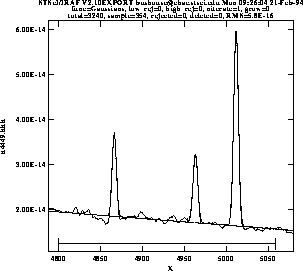
Figure 3.6 shows the results of fitting the H (4861Å) and [OIII] (4959 and 5007 Å) emission features in the spectrum of NGC 4449. The resulting coefficients and error estimates (in parentheses) are shown in Figure 3.7.

Figure 3.6: Fitting H and [OIII] Emission Features in NGC 4449

Figure 3.7: Coefficients and Error Estimates

function = Gaussians 

coeff1 = 8.838438E-14    (0.)            - Baseline zeropoint (fix)  

coeff2 = -1.435682E-17   (0.)            - Baseline slope (fix)  

coeff3 = 1.854658E-14    (2.513048E-16)  - Feature 1: amplitude (var)  

coeff4 = 4866.511        (0.03789007)    - Feature 1: center (var)  

coeff5 = 5.725897        (0.0905327)     - Feature 1: FWHM (var)  

coeff6 = 1.516265E-14    (2.740680E-16)  - Feature 2: amplitude (var)  

coeff7 = 4963.262        (0.06048062)    - Feature 2: center (var)  

coeff8 = 6.448922        (0.116878)      - Feature 2: FWHM (var)  

coeff9 = 4.350271E-14    (2.903318E-16)  - Feature 3: amplitude (var)  

coeff10 = 5011.731       (0.01856957)    - Feature 3: center (var)  

coeff11 = 6.415922       (0.03769293)    - Feature 3: FWHM (var)

rms           = 5.837914E-16 

grow          = 0. 

naverage      = 1 

low_reject    = 0. 

high_reject   = 0. 

niterate      = 1 

sample        =  4800.132:5061.308