Common DFOS tools:
|
||||||
| dfos = Data Flow Operations System, the common tool set for DFO | ||||||
|
![]() make
printable | back to: phoenix description · process instances
make
printable | back to: phoenix description · process instances
| PHO ENIX |
phoenix: instances - MUSE |
Find here a detailed overview of the characteristics of the MUSE PHOENIX process. The focus is on specific properties for MUSE. The standard PHOENIX process is not covered here, find it here. Find the phoenix tool documentation here.
Phases of phoenix process:
MUSE datacubes are big (3-5 GB for single, 3-50 GB for combined ones). Their production is complex, it requires significant resources and compute time. In order to maximize the usefulness for their users, a certain amount of non-standard features is part of the PHOENIX process. The most prominent feature is the non-standard association scheme (called "smart association" with non-OCA rules), combined with the non-standard creation of the science cascade (going beyond what is possible with createAB). You may want to read more about this feature here before you read this section.
The smart association scheme is implemented with the tool phoenixPrepare_MUSE. The non-standard creation of science ABs is implemented with the phoenix pgi called pgi_phoenix_MUSE_AB.
This is a semi-automatic, command-line tool. It is called on the command line, either by date or by month:
phoenixPrepare_MUSE -d <date>
phoenixPrepare_MUSE -m <yyyy-mm>
For a given date, it analyzes the entire set of science headers, evaluating the keys container_id, container_type, obs_id, tpl_start, obs_start, the dpr keys, and keys related to the differential offsets and the rotator angles. It analyzes all datasets defined by the container keys, the obs_id and tpl_start.
First, it checks for containers of type C (concatenated). These might contain two or more linked OBs which would then be evaluated together (this goes beyond the OCA rules). Then it checks for repetitions of the same OB (same night of course), which sometimes happens (both for VM and SM). Finally, it analyzes multi-template OBs, for the operator to decide if they should get combined (stacked) or not (mapping) (more on these patterns here ...).
The relative acquisition pattern of each OB (or container), based on the differential offset values, is visualized by a small MIDAS script.
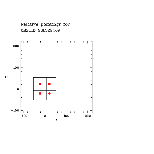 |
Display of acquisition pattern for a given OB, to decide about 'smart association'. The plot displays the centre of each 1x1 arcmin^2 FOV (red dot), plus its boundaries. The example OB has two templates, therefore two ABs. Based on this plot, they get merged into one AB because there is sufficient overlap. |
The design of the tool is such that it takes the science ABs as created by the DFOS account, from http://qcweb.hq.eso.org/MUSE/logs/2014-12-14/. These are either scibasic ABs (single file) or exp_combine ABs (tpl).
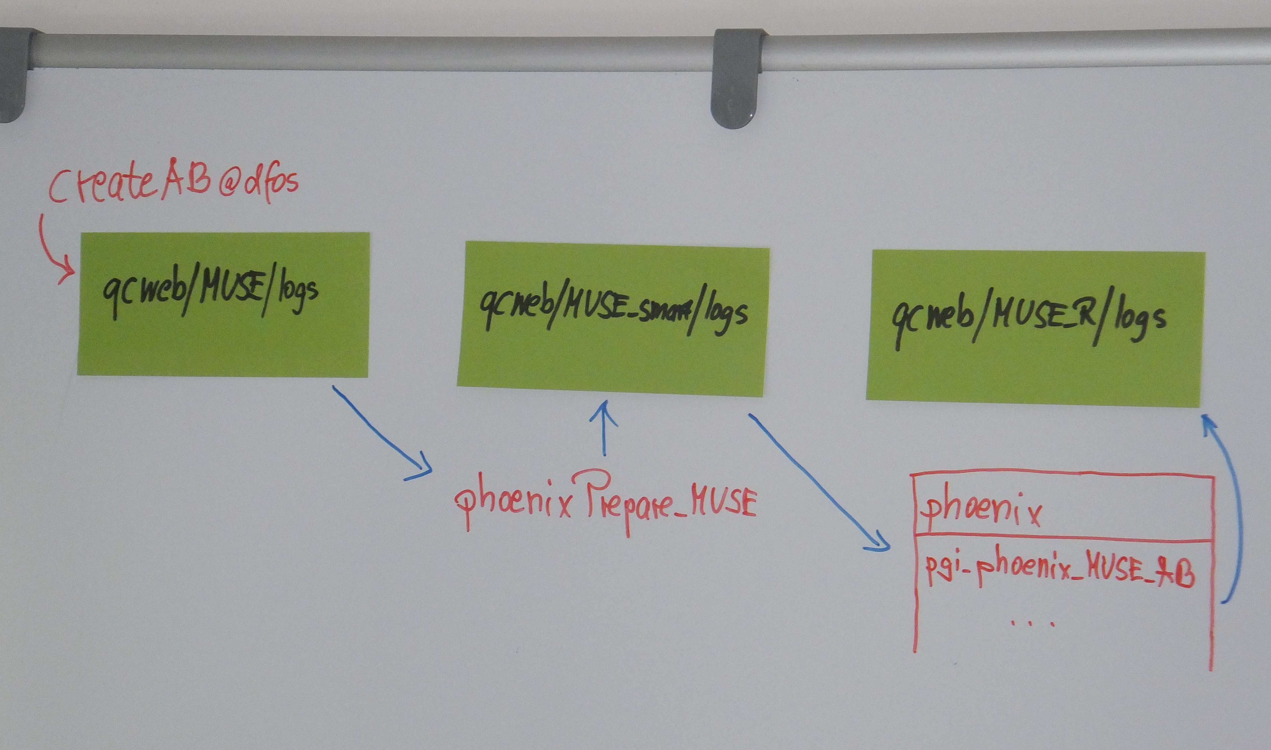
After interaction with the ABs (with or without changes), the resulting ABs are uploaded to a new branch, http://qcweb.hq.eso.org/MUSE_smart/logs/2014-12-14/, for permanent storage. This is where they are later expected by the phoenix tool. Any modification done to the ABs applies to the input datasets only (set of RAWFILEs). All associations to master calibrations are left unchanged. The MUSE_smart directory is a "buffer" to become independent of the DFOS storage, while having a permanent storage of the modified ABs for future reference. All science ABs are stored in the MUSE_smart tree, no matter if they are modified or not. When phoenix is called, it will download the ABs from the MUSE_smart directory. After finishing it will store the ABs under the final tree http://qcweb.hq.eso.org/MUSE_R/logs/2014-12-14/ .
The tool tries to analyze the dataset patterns and offers to the operator a number of (context-aware) actions, among them
These are the most common actions:
| Action | Description |
| MERGE | multi-template ABs can be merged |
| DELETE | for merged ABs, the previous tpl ABs are deleted |
| EDIT | custom editing of datasets |
| SPLIT | ABs can be split by alpha/delta offsets if there is no/little overlap |
| ADD SKY | for 'hidden sky': replace static SKY calibs by SKY products |
| TRANSFORM | for 'hidden sky': transform ABs from SCI_SINGLE to SKY_SINGLE |
All edits are logged in a simple-minded logging system for future reference, in phoenixPrepare_MUSE_2014-12-14.log.
The tool is designed as an "expert system", with more options to be added relatively easily if needed.
As the last step, the tool will transfer, after confirmation, all ABs and ALOG files (no matter if edited or not) to the MUSE_smart tree on qcweb.
Options:
| phoenixPrepare_MUSE -h | quick help about options |
| phoenixPrepare_MUSE -H | executive help |
phoenixPrepare_MUSE -d <date> |
run for specified date only |
| phoenixPrepare_MUSE -m <yyyy-mm> | loop on all dates for the specified month |
| phoenixPrepare_MUSE -S | simulation: only analysis based on headers; no downloads or uploads of ABs |
| phoenixPrepare_MUSE -B | point browser on the daily data list (useful) |
| phoenixPrepare_MUSE -V | interactive mode (recommended, tool waits for confirmation) |
Note:
The principle of SMART association is to review the DFOS ABs, in order to maximize the usefulness of the datacube product. This feature is provided by the pre-processing tool phoenixPrepare_MUSE which must be run before phoenix.
In many cases the standard input data set (RAWFILE) which is based on TPL_START is not changed, but there are typical patterns when it is better to optimize the ABs. Here is an overview of the most common cases.
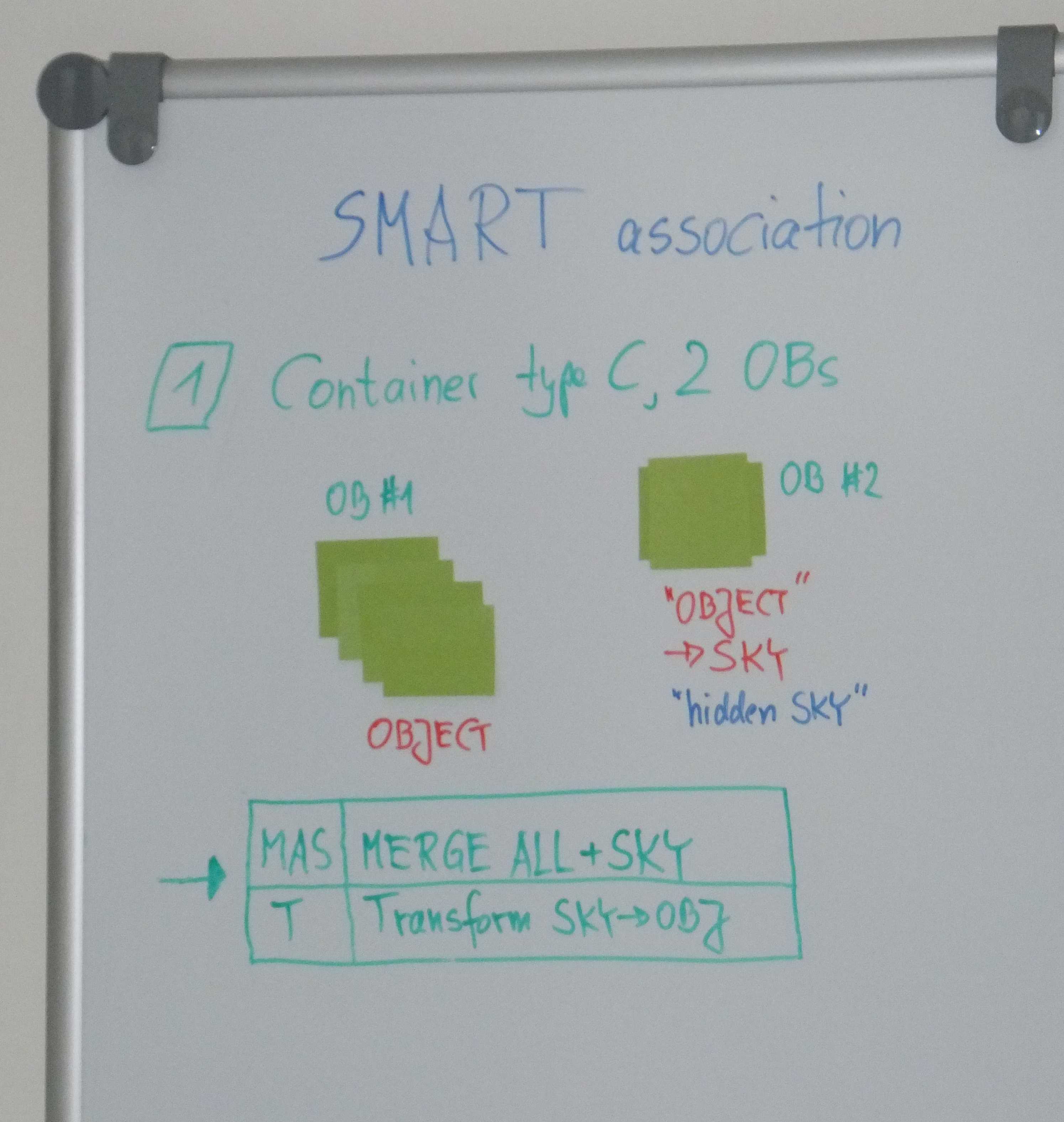 |
Case #1: 2 OBs linked by the same CONTAINER ID (type C). |
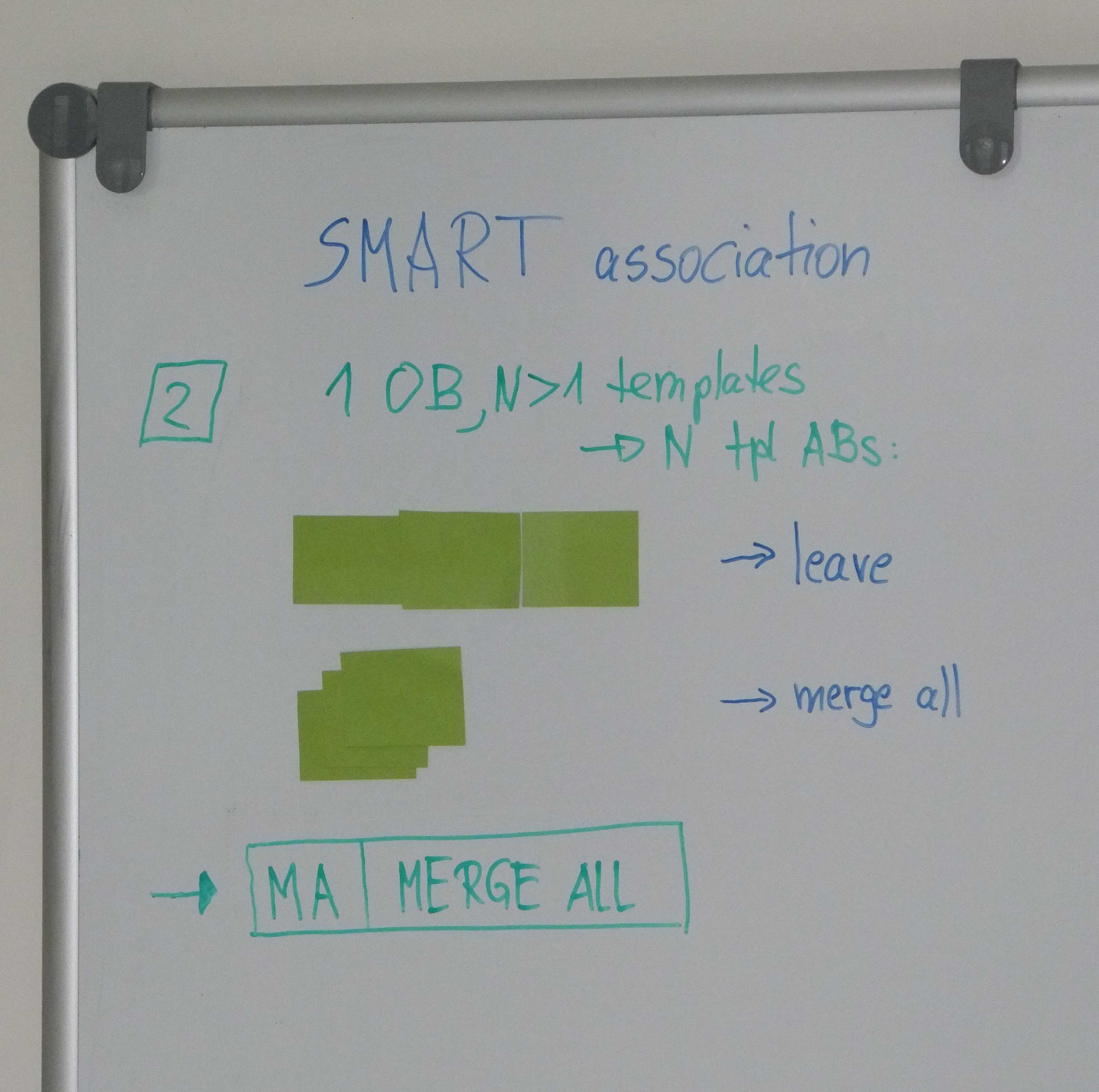 |
Case #2: 1 OB, more than 1 template. Depending on jitter offsets, one might want to merge all tpl ABs. |
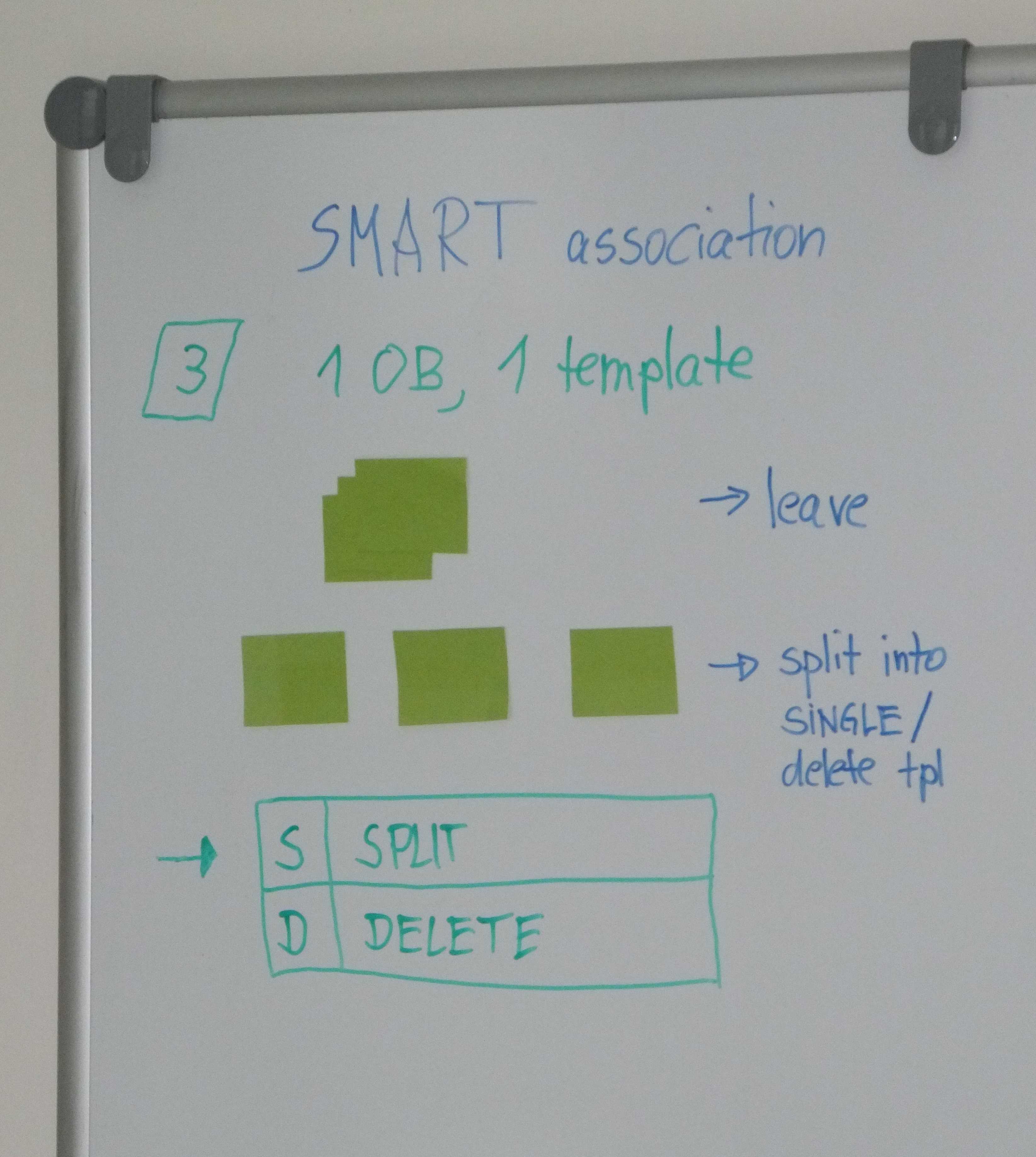 |
Case #3: 1 OB, 1 template. Depending on jitter offsets, one might want to split the tpl AB into smaller datasets, or even delete it (provide single datacubes only) if there is no overlap at all. |
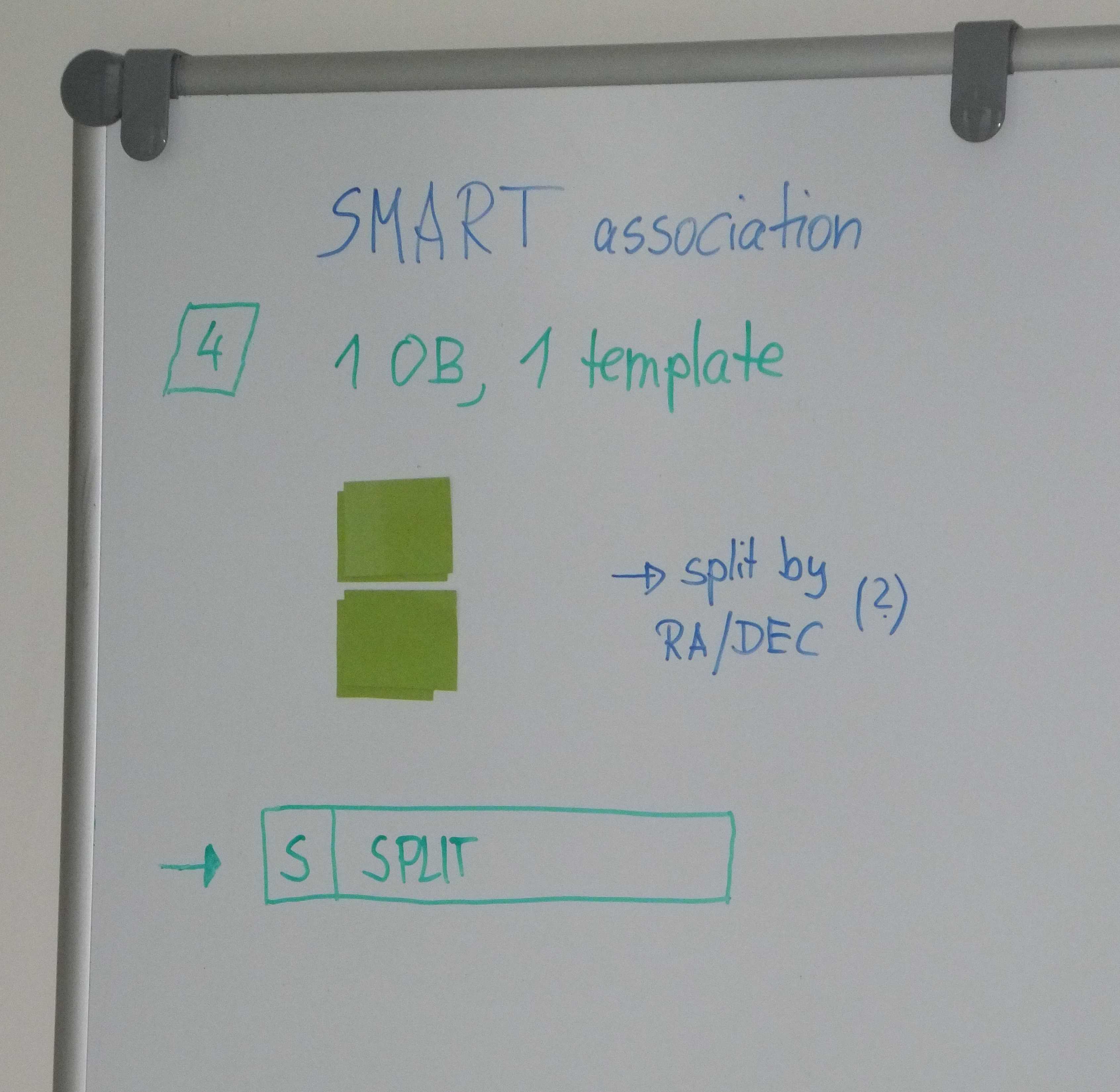 |
Case #4: 1 OB, 1 template. Data come in twins. One may want to split by RA and/or DEC. (This option is likely to be obsolete. With the option to process up to 16 input files, an N=16 combined datacube might still be preferrable over say 8 combined datacubes, each of them made from 2 input files.) |
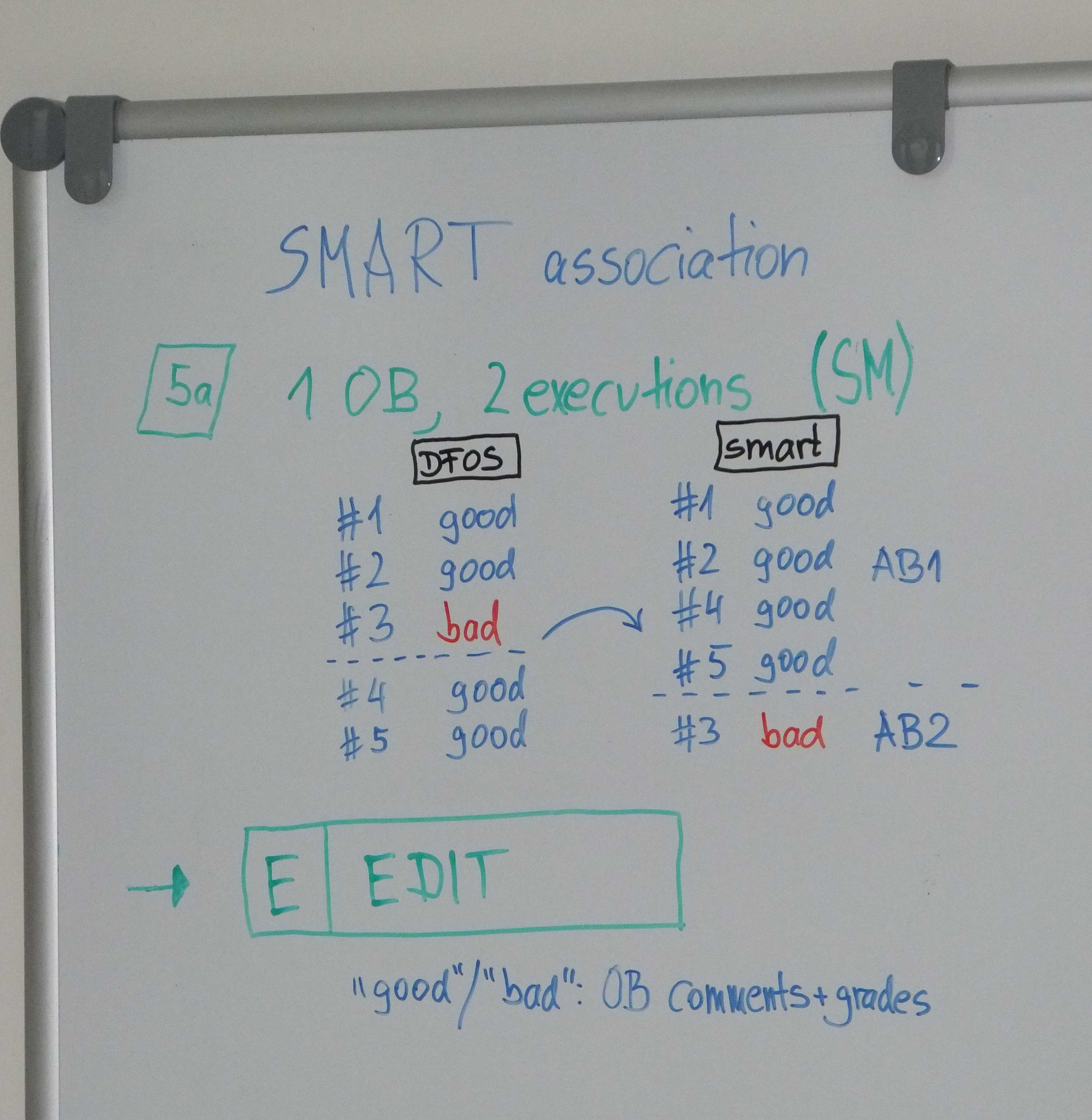 |
Case #5a: 1 OB, 2 executions, the SM case. Based on OB grades and comments, it is often possible to identify the bad file(s) and the good files. By editing, one can create one good tpl AB and one not so good (but still useful) (tpl or single) AB. |
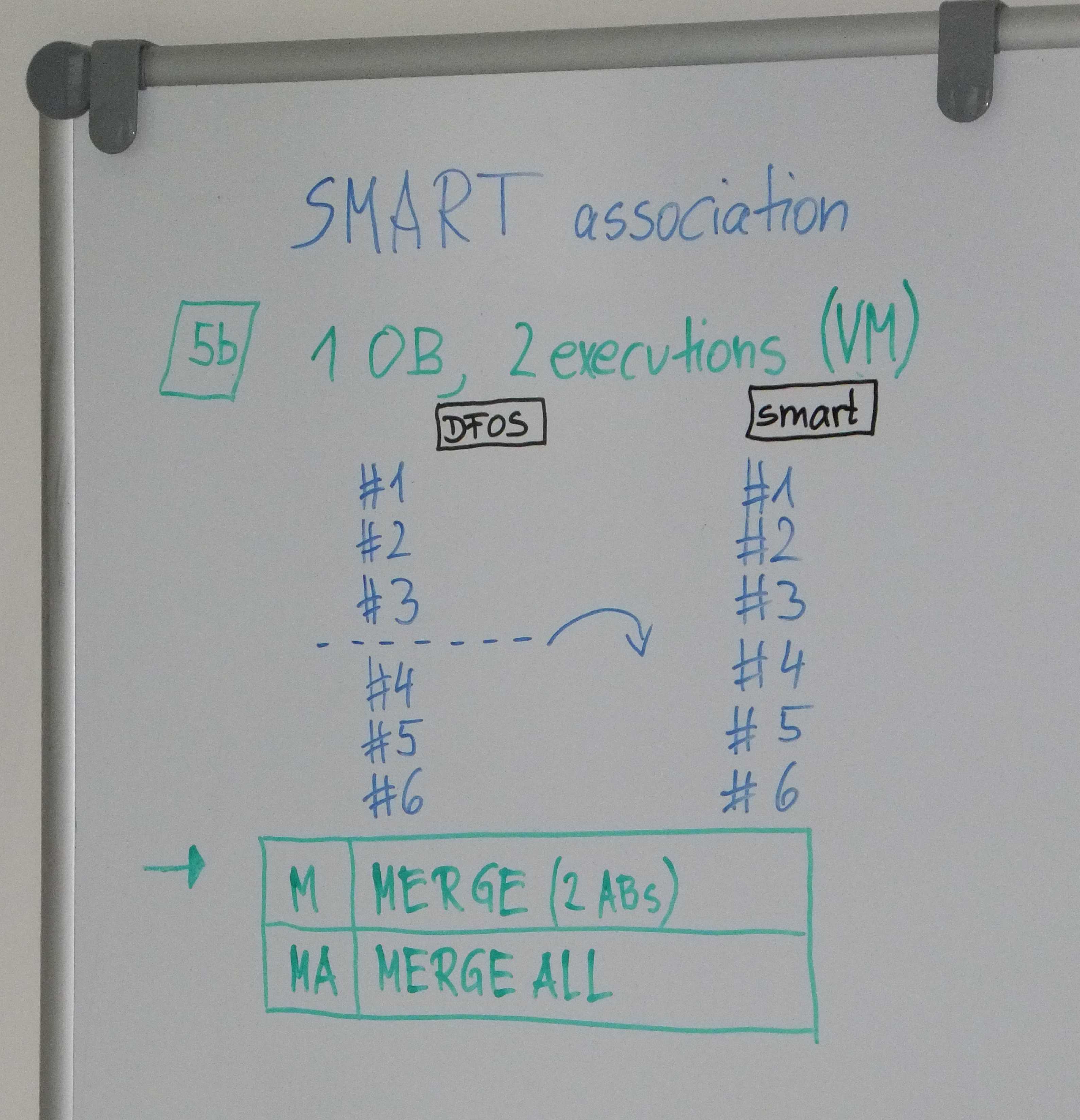 |
Case #5b: 1 OB, 2 executions, the VM case. Typically no OB comments are available. A combination of all executions into a single tpl AB is likely the best option. |
 Processing: pgi_phoenix_MUSE_AB
When working with phoenix for MUSE, always work on single dates. Typical execution times for a full (data) date are fractions of a full (calendar) day. The typical call is
| phoenix -d 2014-12-14 -C | Call the first part of phoenix (AB creation); no execution: ideal for checking and testing |
| or | |
| phoenix -d 2014-12-14 -P | Call the first and the second part of phoenix (AB creation, AB processing, QC reports): the real thing |
Because of the interactive certification step for the MUSE IDP process, it is not possible to call the phoenix tool without option (like phoenix -d 2014-12-14).
The phoenix tool works with standard dfos components plus with instrument-specific PGIs. For MUSE the first PGI is
| pgi_phoenix_MUSE_AB | configured as AB_PGI |
It is needed to create the full science AB cascade with 5 recipes and processing steps. In particular:
| 1 | muse_scibasic | .ab |
| 2 | muse_scipost | _pst.ab |
| 2a | muse_create_sky | _sky.ab |
| 3 | muse_exp_align | _tal.ab |
| 4 | muse_exp_combine | _tpl.ab |
The different types of ABs can be recognized by their extension.
Depending on the number of input frames, and on their type, there are four different cases:
| a) single OBJECT frame, no SKY: | |
 |
Output of PGI: one scibasic AB, and one scipost AB. |
| b) N=4 input OBJECT frames, no SKY: | |
 |
Output of PGI: 4 scibasic ABs, 4 scipost ABs, one exp_align AB, one exp_combine AB. |
| c) N=4 input OBJECT frames, 1 SKY: | |
 |
Output of PGI: 4+1 scibasic ABs, one create_sky AB, 4+1 scipost ABs, one exp_align AB, one exp_combine AB. The additional SKY scipost AB will create a shallow datacube. |
| d) N=4 input OBJECT frames, 2 SKY frames: | |
 |
Output of PGI: 4+2 scibasic ABs, 2 create_sky ABs, 4+2 scipost ABs, 2 exp_align ABs, 2 exp_combine ABs. The SKY ABs will create a shallow combined datacube. |
The creation of scipost, exp_align and exp_combine ABs for SKY files is based on the idea that these are valid pointings and contain science photons ("serendipitous science").
In the process of AB creation (from the "simple" set of ABs delivered by phoenixPrepare_MUSE), the PGI manages
It also manages the content of the ALOG files (for consistency only), and detects and suppresses configured cases of ultra-short exposure times (<10 sec) or excessively high number of input files (> 16 currently).
It does not create new associations.
After execution all ABs are in the standard $DFO_AB_DIR, ready for execution.
Processing: pgi_phoenix_MUSE_stream
The second important PGI is pgi_phoenix_MUSE_stream which is configured as JOB_PGI. This PGI manages the orchestration of the AB execution. Like the AB_PGI implements association functions that are not available in createAB, this JOB_PGI implements dependency functions that go beyond what is possible with createJob.
MUSE AB processing executes without condor. Instead, the pipeline uses internal parallelization, with 24 threads equivalent to the 24 fits file extensions (24 spectrographs). On a powerful machine like muc10 or muc09 (with 48 or 32 physical cores each), it is possible to run 2 such ABs in parallel ("2 streams"). On muc10 one can even go for 3-4 streams. Because of the logical dependencies, the execution scenario is the following:
| type | ext | sequence | streams | why | typical performance |
| scibasic SKY ABs | .ab | 1 | 1 (sequential) | coming first since they are needed subsequently in scibasic OBJECT ABs; memory intensive | 3-5 min |
| create_sky ABs | _sky.ab | 2 | 1 | needs output from #1 | 3-5 min |
| scibasic OBJECT ABs | .ab | 3 | 2 or 3 | need output from #2 (if existing); memory intensive, can go in 2 (or more) streams for performance | 3-5 min |
| scipost ABs (SKY or OBJECT) | _pst.ab | 4 | 2 or 3 | output from #3 needed; only partly multi-threaded, can go in 2 (or more) streams for performance | 10-30 min |
| exp_align ABs | _tal.ab | 5 | 1 | output from #4 needed; very quick | <1 min |
| exp_combine ABs | _tpl.ab | 6 | 1 | output from #3 and #4 needed; can become memory intensive, hence only 1 stream | 20-200 min |
For performance reasons, independent ABs are executed in 2 or more streams whenever possible (and safe). For a complete daily batch, the ABs are sorted and executed in the following manner (time from left to right):
| type of ABs: | scibasic OBJECT .ab |
scipost _pst.ab |
||||
| scibasic SKY .ab |
create_sky _sky.ab |
exp_align _tal.ab |
exp_combine _tpl.ab |
|||
| scibasic OBJECT .ab |
scipost _pst.ab |
|||||
| job file: | execAB | JOB_MANAGER | execAB | |||
time  |
[split] | [merge] | ||||
If there are no SKY AB, we start with the OBJECT ABs in 2 or more streams. If there are no combined ABs, we finish with the streams of scipost ABs. There are always the 2 or more streams for the OBJECT ABs.
There are two critical points in the flow: the splitting into multiple streams after the _sky ABs ('split point'), and the merging into one stream before the _tal ABs ('merge point', see above). This is controlled in the following way:
This last transition to single-stream processing is done for safety: we do not precisely know how many input pixeltables are going to be combined in the last step. Per input pixeltable, about 20-25 GB memory is required. For combing N=4 pixeltables (the standard case) we would need up to 100 GB which would be safe in 2 or even 3 streams (both mucs have 512 GB each). But there are occasionally larger jobs, hence we stay safe and process only one stream. (If the machine runs out of memory the job eventually fails, after hours of swopping.)
As said above, the number of supported parallel streams differs for the operational machines. It is configured in config.phoenix as 'MULTI_STREAM' and is 2 on muc09, and 3 on muc10 (but check for the correct values there).
In order to get familiar with the processing pattern, call 'phoenix -d <date> -C' which not only gives you the complete set of ABs, but also the execAB and the JOB_MANAGER files.
The sequence of QC jobs is listed in the standard way in the execQC file. There is one job per pst and tpl AB. They are executed in sequence. Their execution time is about a minute each and does not need optimization.
-- ... the tal (exp_align) AB fails, causing the tpl (exp_combine) AB to fail:
-- ... a set of scibasic or scipost ABs failed because of NGAS access problems:
Certification: phoenixCertify_MUSE
After finishing the 'phoenix -P' call, the products are (as usual) in $DFS_PRODUCT, waiting for certification. This step is special for MUSE, no other IDP process has a strict review phase. It is deemed necessary because there are potential issues:
The certification tool phoenixCertify_MUSE is configured as CERTIF_PGI. It is a clone of certifyProducts, customized to the MUSE IDP needs. It can be called stand-alone on the command line, but normally it is called by the third step of phoenix, after processing:
| phoenix -d 2014-12-14 -M | Call the third part of phoenix (certification, moveProducts) |
It has the same workflow as the dfos tool. It has some hard-coded configuration, like RANDOM mode (20%) for the SCI_SINGLE products (from pst ABs), and ALL mode for the PIXTABLE_REDUCED products (from tpl ABs). Since the review is score-supported, the RANDOM mode means exactly the same as under DFOS: at least 20% of all products are reviewed, plus the non-zero scores, plus the failures. There is the usual comment mechanism. Note that the products of the tpl ABs have already auto-edited their PATTERN as QC comment (acquisition pattern). It is not possible to jump, but QC comments can be entered anytime using the 'pgi_phoenix_MUSE_getStat' link on top of the AB monitor.
To assist with the review, the OB comments and grades are displayed throughout the certification.
Apart from the PATTERN, there are auto-comments on the AB monitor if the pipeline log contains WARNINGs or ERRORs, and if the datacube is a SINGLE one. (These auto-comments are meant for information; they don't get propagated but are overwritten by the certification procedure.) Please check the logs for better understanding. The following standard ERRORs are known:
If you encounter a PATTERN 'unknown', the QC script has not found a proper value for the observed pattern. Though this is not an issue, you may want to improve the script and make the new pattern known to it:
If you want to enter a comment about a specific pst AB, use the 'pgi_phoenix_GEN_getStat' button on top of the AB monitor. Because of the hard-coded 20% fraction of reviewed ABs, there is no guarantee that the certification tool will offer that specific AB for review (unless it scores red of course).
The MUSE QC system has the following components:
All follow the standard DFOS scheme.
QC procedures. There are two QC procedures (both under $DFO_PROC_DIR):
(note: the names are historical, they have no proper meaning). Both are largely similar but differ when dealing with the additional properties for the combined datacubes (products of tpl ABs). They feed the QC parameters into the QC1 databases, derive the score bit, and call the python procedure for the QC plots. The qc1Ingest calls for the QC1 parameters are stored locally, under $DFO_PROC_DIR, as qc1_PIXTABLE_OBJECT/REDUCED.dat and qc1_sources.dat. There is also a technical table qcpar_PIXTABLE_OBJECT.dat that is used for the PATTERN recognition (originally it had other functions but these faded away).
QC parameters, QC databases. The QC parameters are generally speaking all kinds of parameters that might be useful, not only for QC, but also for process monitoring (e.g. PATTERN, score_bit), research on science cases (PROG_ID, abstract links) etc. They are fed into three QC1 databases:
The first two are rather similar in structure and collect data for the single and combined datacubes. The third one collects parameters for every pipeline-identified source and could be used to monitor alignment quality etc.
Scoring system. The are two aspects of the scoring system:
There are 7 scores for single datacubes (pst ABs):
There are 4 scores for combined datacubes (tpl ABs):
Since the MUSE pipeline is very "tolerant" with failures at intermediate steps (where other pipelines would just fail), it seems useful to monitor e.g. the size of the output datacube, or check for complete processing.
While the output of the scoring system is used for certification, and is stored locally but not exported to the user, the score_bit is used to give the user some indication about the data quality. It consists of 11 binary values (0 or 1) coding product properties in a very concise way. They are documented here and in the release description. They are automatically derived by the QC system and written into the product headers as key QCFLAG.
QC plots. Each product datacube gets its QC plot which is ingested into the phase3 system and gets delivered to the user. They are created by the python routine muse_science.py under $HOME/python.
Post-processing: pgi_phoenix_MUSE_moveP
After certification the standard phoenix workflow takes place (calling moveProducts). There is a pgi within moveProducts, pgi_phoenix_MUSE_moveP, that controls the complex final distribution of the datacube products:
This delivery plan makes sure that all final datacubes (last processing step) are delivered as IDPs, that all combined datacubes have the individual datacubes downloadable on demand, and that all IDPs have a preview file (IMAGE_FOV).
After phoenix: conversion tool idpConvert_mu and ingestProducts
After phoenix has finished, all science products are in $DFO_SCI_DIR, all logs in $DFO_LOG_DIR, and all graphics in $DFO_PLT_DIR. This is the standard architecture also known from DFOS.
The final call is 'ingestProducts -d <date>' which for MUSE has three parts:
In order to prepare for IDP ingestion, the single datacubes need to be dpIngested (if applicable), and IDP headers need to be modified. This is the task of idpConvert_mu. (Every IDP process has such an instrument specific tool, with the instrument coded in its name).
| idpConvert_mu -h | -v | call help , get version |
| idpConvert_mu -d <date> | call the tool for a given date |
| idpConvert_mu -d <date> -C | do a content check (check for completeness of all science and ancillary files) and exit |
The tool checks first if
The ingestion log is in the usual place known from dfos: $DFO_LST_DIR/list_ingest_SCIENCE_<date>.txt.
The files get ingested as 'S.' files. You can check their existence by calling 'productExplorer -d <date>'. They will display in blue.
These files are ingested 'just in case', for an archive user who discovers issues with the combined datacube and then wants to inspect the individual ones. Their names get registered in the header of the IDP, before ingestion.
Next, the conversion tool adds ASSOC, ASSON and ASSOM keys to define the IDP dataset, consisting of the IDP (datacube), its ancillary fits file (IMAGE_FOV), ancillary text file (pipeline log), and ancillary graphics (QC reports). See more in the release description.
After finishing, the tool has
The products are then ready to be phase3-ingested with ingestProducts.
The call of ingestProducts and, afterwards, cleanupProducts is usually done in the same way as known from DFOS_OPS:
The successful ingestion is displayed on the phoenixMonitor.
Note that for MUSE there is the CLEANUP_PLUGIN needed (pgi_phoenix_MUSE_cleanup) that
There is a number of little tools for all kinds of special tasks. If possible they were configured with standard mechanisms in the standard DFOS tools or in phoenix. Their naming scheme follows a standard when they are specific for phoenix: they start with pgi_phoenix, then follows either MUSE or GEN. Unless otherwise noted, they are stored in $DFO_BIN_DIR.
| phoenixGetLogs | Collects all pipeline log files for a final datacube; the output is a text file called r.MUSE...log and is stored in $DFO_SCI_DIR/<date>, for final ingestion along with the IDPs. The tool is called by pgi_postSCI (for pst and tpl ABs) which is the post-processing plugin for processAB. |
| pgi's for processAB: | |
| pgi_preTPL | for tpl ABs only: corrects sequence of input files according to timestamp (SOF_CONTENT, MCALIB); relevant for tpl ABs since the combined datacube inherits mjd_obs from the first input file in the list. |
| pgi_postSCI | provides a number of actions at the end of processAB:
|
| pgi_phoenix_MUSE_postAB | FINAL_PLUGIN of processAB; used to
|
| pgi's for phoenix: | |
| pgi_phoenix_MUSE_AB | AB_PGI; controls the science cascade; see here |
| pgi_phoenix_GEN_MCAL | HDR_PGI; checks for unsuccessful mcalib downloads |
| pgi_phoenix_MUSE_stream | JOB_PGI; creates the job files for multi-stream processing; see here |
| phoenixCertify_MUSE | CERTIF_PGI; provides the certification of MUSE science products; see here |
| other tools/pgi's: | |
| phoenixMonitor | standard phoenix tool, configured for MASTER/SLAVE model (see dual-instance processing). |
| pgi_phoenix_MUSE_getStat | offers a dialog for comment editing per AB, useful in certification step (plugin for getStatusAB) |
| pgi_phoenix_MUSE_moveP | SPECIAL_PLUGIN for moveProducts; manages the distinction between final datacubes (go to $DFO_SCI_DIR/<date>) and single datacubes (go to $DFO_SCI_DIR/DPING/<date>). |
| pgi_phoenix_MUSE_postQC | PGI_COVER and FINAL_PLUGIN for processQC; provides:
|
| pgi_phoenix_MUSE_renameP | SPECIAL_PLUGIN for renameProducts; checks for "unknown PRO.CATG" messages in the renaming process; was useful in the initial phase, now probably obsolete. |
| pgi_phoenix_MUSE_cleanup | CLEANUP_PLUGIN for ingestProducts; manages the header replacement of all fits files and the header transfer to the MASTER machine (see below) |
| Stored in $DFO_PROC_DIR: | |
| general_getOB.sh | tool to retrieve the OB grades and comments from the database; called by phoenixPrepare_MUSE and by pgi_phoenix_MUSE_AB; the output is stored in $DFO_LOG_DIR/<date> in ob_comments and ob_grades. These files are read by several other tools, among them idpConvert_mu; their content is written into the IDP headers. |
Multi-instance processing (MASTER/SLAVE model)
Even for the 48-core machine muc10, the MUSE datacube production line is very time-consuming and demanding. The data processing for a day worth of MUSE science data might take half a day or more of machine time. This is very different to all other IDP processes (the other extreme being UVES where the whole IDP dataset could in theory be reprocessed over a long weekend).
Hence a multi-instance processing model has been developed which uses more than one muc machine (muc10 and muc09; at times also muc11, muc12):
| muc10 | muc09* | |
| muse IDP account | muse_ph2 | muse_ph (ph stands for 'phoenix') |
| role | MASTER | SLAVE |
| physical processors | 48 | 32 |
| memory [GB] | 512 | 512 |
| slot (UT) | 0-24 | 17-07:54 |
| data disk [TB] | 10 | 3.5 (50% quota of 7 TB) |
The accounts work largely independently (you can of course run a phoenix job on muc09 and another one on muc10). But when it comes to store the output (headers of fits files, logs, plots, statistics), we use a MASTER/SLAVE model: all information is ultimately stored centrally, on the MASTER, so that the phoenixMonitor running there collects the information about the entire process (no matter if processed on the MASTER or on any SLAVE), just like on any other 'normal' IDP account. This means that information is scopied from the SLAVE to muc10 (MASTER) (but never in the other direction).
Software. All accounts share the same tools and configuration files (with a few keys filled with account-specific information). The accounts are coupled via the ssh mechanism to easily exchange information.
All accounts run a daily cronjob of dfosExplorer. It is the responsibility of the operator to keep them up-to-date in the same way. The non-dfos tools (MUSE-specific pgi's) are not covered by this mechanism. They need to be carefully kept in sync by the operator. Good practice is to use muse_ph2@muc10 as the logical MASTER: any changes done here are then scp'ed to the SLAVE account.
Both accounts run a weekly cronjob of dfosBackup.
Output. The phoenix processes run independently up to the step of finishNight, after which the SLAVE scopies logs and plots to the MASTER (same directories on both accounts). This is important for central bookkeeping via phoenixMonitor: only the instance running on the MASTER has the full knowledge and is allowed to export to qcweb.
Ingestion. All fits files are kept in the respective $DFO_SCI_DIR directories (copying would take a long time), and ingest from there. Once ingested, the fits files are ultimately deleted by cleanupProducts. At that point the headers are transferred from the SLAVE to the MASTER.
The config file of phoenix is used to define the roles of the account (keys IS_SLAVE and MASTER_ACCOUNT).
Scheduling. Unless for other IDP instances, there is no explicit scheduling mechanism for the phoenix jobs of MUSE (because the monthly mode cannot be used for MUSE). A MUSE phoenix job is always launched manually. It is the responsibility of the operator to decide which dates are to be launched. There is a notification mechanism implemented on the MUSE DFOS machine muc09, that adds a JOBS_NIGHT entry on muc10 when a night with SCIENCE data is dfos-finished. This is inteneded as a reminder mechanism that eventually the corresponding phoenix should be executed.
History: http://qcweb/MUSE_R/monitor/FINISHED/histoMonitor.html
Release description: under http://www.eso.org/sci/observing/phase3/data_streams.html.
Monitoring of quality: automatic scoring system, with a dedicated qc1 database table. See also here.
| Final datacube | All science raw files are processed into a single datacube. Many of them are then combined into a combined datacube. The combined datacubes are always final datacubes, but there also cases when a single datacube is not processed further, then it runs into a final datacube as well. All final MUSE datacubes become IDPs. Cases when a single datacube becomes a final datacube:
|
| Hidden sky | Some concatenated OBs are designed to contain, in the easiest case, 1. the OBJECT OB, with standard and correct DPR keys, and There might also be more complex cases, like 5 OBs with single exposures in one CONTAINER all claiming to be OBJECTs, but with 3 being (identical) OBJECT pointings and 2 hidden sky. The tool phoenixPrepare_MUSE recognizes these two cases (but there might be more in the future). It lets the user mark the OBs properly and then edits the corresponding ABs correctly. |
| PATTERN | The QC script for the PIXTABLE_REDUCED products (of the tpl ABs) evaluates the acquisition pattern of the combined datacubes. Here are some values. The QC1 database has all possible values listed (http://archive.eso.org/qc1/qc1_cgi?action=qc1_browse_table&table=muse_sci_combined). The PATTERN is also displayed on the coversheets. It helps understanding the OB design and is e.g. useful to confirm the decisions made with phoenixPrepare_MUSE. PATTERNs come as:
PATTERN can also be SINGLE. |
| Score bit | Simple-minded way of transfering the scoring information to the end user. A score bit is a binary value with 9 flags (for single cubes) or 11 flags (combined cubes). They are written as key QCFLAG into the IDP headers. Find their definition here. |
| Shallow datacube | The creation of scipost etc. ABs for SKY files is based on the idea that these are valid pointings and contain science photons ("serendipitous science"). In many cases they have shorter exposure times than OBJECT frames and hence are called "shallow cubes". As the OBJECT cubes, they might come as single or as combined datacubes, depending on the OB design. |
| Smart association | Review the standard input data set (RAWFILE) which is based on TPL_START. For MUSE it is important to maximize the usefulness of the datacube product. Smart association takes also into account: containers, "hidden sky" OBs, incomplete/aborted OBs, multiple-execution OBs. It attempts to revise the dataset in various ways:
Find more information here. |
| Last update: April 26, 2021 by rhanusch |