Deployment, Tuning, Benchmarking & Troubleshooting

In this chapter some information in connection with the installation and usage of the FGF Package are provided.

Installation

The FGF is normally installed in the “/elt” root as other IFW components, on a standard IFW machine. If necessary new versions can be installed on the machine via RPMs, if such are available. If no recent RPM is available, it is possible, as usual, to install it directly from Gitlab.

The only other IFW component, used by FGF, is IFW Foundation Component (“ifw-fnd”).

Deployment Setup

The procedure of creating a new FGF Application is described in detail in Creating an FGF Application: Creating an FGF Application.

Before creating the new FGF Application, it shall be determined how to deploy it:

As a standalone application, usually on a dedicated FGF Node (like an embedded system).

As an application on the IWS, normally part of the instrument main NOMAD execution environment.

On a dedicated, higher-level auxiliary IWS, deployed e.g. for load balancing.

Possibly other scenarios might be relevant.

For option 1., the new FGF Application should be created with as a Standalone FGF Application (see Creating an FGF Application: Creating an FGF Application).

For option 2. and 3., the new FGF Application might be integrated as a subsystem into the overall Instrument Tree.

Note

It shall be stressed here, that if spefic SW, normally a proprietary SDK, and/or dedicated HW is needed to interface with the camera, option 1. above, must be applied, since it is not desirable to make the IWS dependant on 3rd party SW and HW.

Regarding selecting the deployment HW, i.e., the FGF Node, the FGF Project does not provide a specific list of HW to choose from, as this is difficult to maintain and requirements from the various projects may differ.

Some guidelines in this context are:

The chosen node shall be industrial grade and ‘ruggedised enough’ to endure deployment in the operational environment, ensuring a long life span.

Ideally, the unit should be easy to mount, e.g., in one of the instrument’s electronics racks if required.

The unit shall have a low power footprint, less than ~30 W (the projects may have specific needs).

The unit shall be fanless, possibly support liquid cooling. If not supplied with direct support for liquid cooling, it shall be considered how this can be achieved to avoid too much heat dissipation from the unit.

It shall be possible to install the standard and most recent ELT Development Environment on the node.

It shall be possible to install and use the necessary HW and SW (SDKs) components on the node.

Consideration shall be given to purchasing hot spares for the unit and addressing long-term obsolescence handling of the unit.

It is acceptable that the new FGF Application is not compiled on the IWS and is not tested e.g. in the Jenkins environment.

In the optimal case, after the commisioning of the instrument, the FGF Application + FGF Node, shall be seen as an embedded solution (=black box) and never touched again, througout the lifetime of the instrument.

This is an example of an FGF Node, in use for the ELT PDS Project:

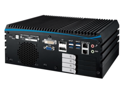
The main characteristics of this unit are:

Model ECX-1320A from vendor Vecow (Plug-in Electronic GmbH).

Fanless, ‘industrial’ PC.

Intel Xeon I5-9500TE CPU, 6 x 2.2 GHz.

PCIe card 10Gb SFP -2 channels (FE-1071).

PCIe card CoaXPress 4 Lane CXP-6 (BitFlow).

8 GB RAM.

500 GB SSD.

Again, the reason for showing this, merely is merely to present an example, and the projects are encouraged to analyse which solution is most suitable for their needs. The projects may of course inquire a list of FGF Nodes already in use by ESO as input for this process.

Software Deployment

This section provides some SW deployment scenarious which might be useful to gain experience with the FGF Framework and which may be useful for troubleshooting. These software deployment scenarios, should be available on a standard ELT DevEnv node.

Test Scenario/Example 1: FGF Simulator + CCF ENVision

The first ready-to-use scenario involves running the FGF Simulator and the CCF ENVision executable.

To make use of this scenario, the following processes should be running on the machine.

The DDT Broker, started with the right command line options (“ddtBroker”).

FGF Simulator (“fgfSim”).

CCF Envision Control Application (“ccfCtrlEnvision”).

Optional: The CCF GUI to facilitate operation of CCF Control (“ccfGui”).

A DDT Viewer, started with the proper command line options (“ddtViewer”). This can be started from the CCF GUI, if used.

The command lines to start each of these are as follows:

DDT Broker:

$ nohup ddtBroker --uri zpb.rr://*:12011/broker &> /dev/null &

FGF Simulator:

$ fgfSim -a 127.0.0.1 -p 59000 -n 127.0.0.1 -s /elt/ifw/resource/image/ifw/ccf/control/test_naxis3_1_512_int16.fits -l ERROR

CCF ENVision Control Applicaton:

$ ccfCtrlEnvision -c config/ifw/ccf/protocols/envision/envision.cfg.yaml -l ERROR -v

CCF GUI:

$ ccfGui -u zpb.rr://127.0.0.1:12092 &

DDT Viewer:

$ ddtViewer -l zpb.rr://127.0.0.1:12011/broker/Broker1 -s rtms-test &> /dev/null &

It is also possible to deploy the UA Expert in parallel to CCF ENVision, to monitor the status directly at the FGF level.

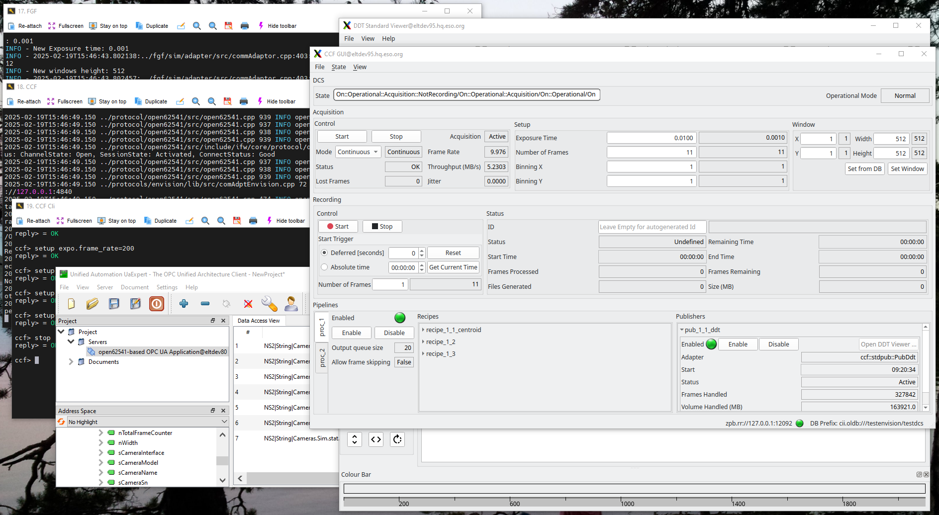
Note again, the DDT Viewer can be started from the CCF GUI. After starting up the processes, it should possible to bring CCF ENVision Control to “Operational::Idle” State, by submitting the “Init”, “Enable” commands. Subsequently “Start” command can be submitted to bring the state to “Operational::Acquisition”. The command can be executed from the CCF GUI. It should now be possible to see images being updated in the DDT Viewer and e.g. store (record) images into FITS files.

The command lines above are meant as examples. E.g., some processes shown, are started in foreground, but it is of course possible to start them in background as well. It is also possible to start with other debugging levels.

The following screenshoot shows an example of the test environment as described above:

To analyse the performance of this setup and the RTMS traffic consult the sections below for more details:

Internal frame handling latency: Internal FGF Application Latency Measurement.

External latency: PerformanceMeasurement.

Analysing UDP traffic using Wireshark: Using Wireshark to Capture and Analyse RTMS Communication.

General network traffic analysis: Other Tools & Means for Network Traffic Analysis.

It would be possible to deploy on two different nodes, but this will require that some configuration parameters are updated accordingly, as the example is meant for a local deployment, on one node, using the loop-back network interface.

Test Scenario/Example 2: FGF Simulator + RTMS Tools - RTMS to DDT Gateway

A more lightweight setup is to only start the FGF Application, e.g. the FGF Simulator, and the IFW RTMS Tools RMTS to DDT Gateway:

Start DDT Broker, if not running:

$ nohup ddtBroker --uri zpb.rr://*:12011/broker &> /dev/null &

Start the FGF Simulator:

$ fgfSim -a 127.0.0.1 -p 59000 -n 127.0.0.1 -s /elt/ifw/resource/image/ifw/ccf/control/test_naxis3_1_512_int16.fits -l ERROR

Start the RTMS Tools RTMS-to-DDT Gateway:

$ rtmstoolsRtms2Ddt -a 127.0.0.1 -p 59000 -w 512 -e 512 -t Int16 --broker-uri zpb.rr://127.0.0.1:12011/broker/Broker1 -s rtms-test -l INFO

Start the DDT Viewer:

$ ddtViewer -l zpb.rr://127.0.0.1:12011/broker/Broker1 -s rtms-test

In order to start the image acquisition, the “uacall” command line tool can be used, or any other OPC UA client:

$ uacall -u opc.tcp://127.0.0.1:4840/ -n "ns=2;s=Cameras.Dvc" -m "2:Start"

This is a simpler setup, which makes it possible to verify the RTMS data received and to test an FGF Application, e.g. while it is being developed, without having CCF in between.

For information about how to analyse the RTMS traffic, refer to the following sections.

System Tuning & Benchmarking

In this section information about how to measure and assess the performance of an FGF Setup is provided.

Internal FGF Application Latency Measurement

It is possible to trigger FGF to measure the internal latency of the frame/packet handling.

The following is computed:

Statistics for sending first packet (latency, stddev, variance, number of samples).

Statistics for sending frame (ditto).

This is an example of how to enable this (from the FGF Simulator):

short CommAdapter::Start() {

    LOG4CPLUS_INFO(m_logger, fmt::format("{}: Starting camera acquisition (Acq Active: {})",
        IFWLOC, m_acq_active));

    if (m_acq_active) {
        return 0;
    }

    m_publisher.ComputeLatency();
    m_publisher.ResetLatency();

    . . .

The following code snippet shows how to retrieve the accumulated stastistics:

short CommAdapter::Stop() {

    . . .

    if (m_publisher.GetComputeLatency()) {
        double latency, stddev, variance;
        int samples;

        m_publisher.GetFirstPacketSentLatency(latency, stddev, variance, samples);
        auto msg = fmt::format("{}: Stats for last acq seq/first packet sent: latency: "
            "{:.3f} micros, stdev: {}, variance: {}, samples: {}", IFWLOC, 1e6 * latency,
            stddev, variance, samples);
        LOG4CPLUS_INFO(m_logger, msg);

        m_publisher.GetFrameSentLatency(latency, stddev, variance, samples);
        msg = fmt::format("{}: Stats for last acq seq/frame sent: latency: "
            "{:.3f} micros, stdev: {}, variance: {}, samples: {}", IFWLOC, 1e6 * latency,
            stddev, variance, samples);
        LOG4CPLUS_INFO(m_logger, msg);
    }

    . . .

    return 0;
}

It shall be noted, when the latency computation is enabled, this will result in a minimal consumption of a few CPU cycles. This however, is so insignificant that it can be disregarded. When disabled, this feature does not take up any CPU cycles.

Troubleshooting

In this section, information about how to perform troubleshooting on a mal-functioning FGF Setup is provided.

It shall be mentioned here, that troubleshooting RTMS applications (in general UDP traffic-based application), might be a bit ‘tricky’, since the amount of traffic may be huge and it may be difficult to locate the origin of the issue.

Using Wireshark to Capture and Analyse RTMS Communication

A useful tool to analyse the UPD traffic on the network or within a node, is the 3rd party application “Wireshark”. Wireshark is installed as a standard application on nodes with the ELT Development Environment installed.

Note

Wireshark may not be used at ESO premises without explicit permission from ESO IT.

The “Wireshark” tools must be run as user “eltdev”on the ELT machines.

In order to use Wireshark to analyse the UDP traffic, the first step is to capture a time series of UDP packet, while an FGF Application is publishing images via RTMS. To do this, invoke the “tshark tool”, e.g.:

eltdev $ tshark -i lo -c 1000 -w fgf.pcap
Capturing on 'lo'
** (tshark:4139529) 17:58:41.237301 [Main MESSAGE] -- Capture started.
** (tshark:4139529) 17:58:41.237344 [Main MESSAGE] -- File: "fgf.pcap"
1000

The proper network interface shall be specified. For this example, the FGF Application is running locally, using the loopback interface. Retrieve the network interfaces using the “ifconfig” command:

$ ifconfig
ens192: flags=4163<UP,BROADCAST,RUNNING,MULTICAST>  mtu 1500
        inet 134.171.2.171  netmask 255.255.255.0  broadcast 134.171.2.255
        ether 00:50:56:91:9e:bd  txqueuelen 1000  (Ethernet)
        RX packets 64399565  bytes 35879871448 (33.4 GiB)
        RX errors 0  dropped 2062  overruns 0  frame 0
        TX packets 21963419  bytes 72554825183 (67.5 GiB)
        TX errors 0  dropped 0 overruns 0  carrier 0  collisions 0

lo: flags=4169<UP,LOOPBACK,RUNNING,MULTICAST>  mtu 65536
        inet 127.0.0.1  netmask 255.0.0.0
        inet6 ::1  prefixlen 128  scopeid 0x10<host>
        loop  txqueuelen 1000  (Local Loopback)
        RX packets 160938938  bytes 433071479495 (403.3 GiB)
        RX errors 0  dropped 0  overruns 0  frame 0
        TX packets 160938938  bytes 433071479495 (403.3 GiB)
        TX errors 0  dropped 0 overruns 0  carrier 0  collisions 0

In a file named e.g. “rtms.lua” store the following information to dissect the UDP traffic captured by “tshark”:

local udp_table = DissectorTable.get("udp.port")
local mudpi_proto = Dissector.get("mudpi")
udp_table:set(59000, mudpi_proto)
local mudpi_table = DissectorTable.get("mudpi.topic_id")
local rtms_proto = Dissector.get("rtms")
mudpi_table:set(10, rtms_proto)

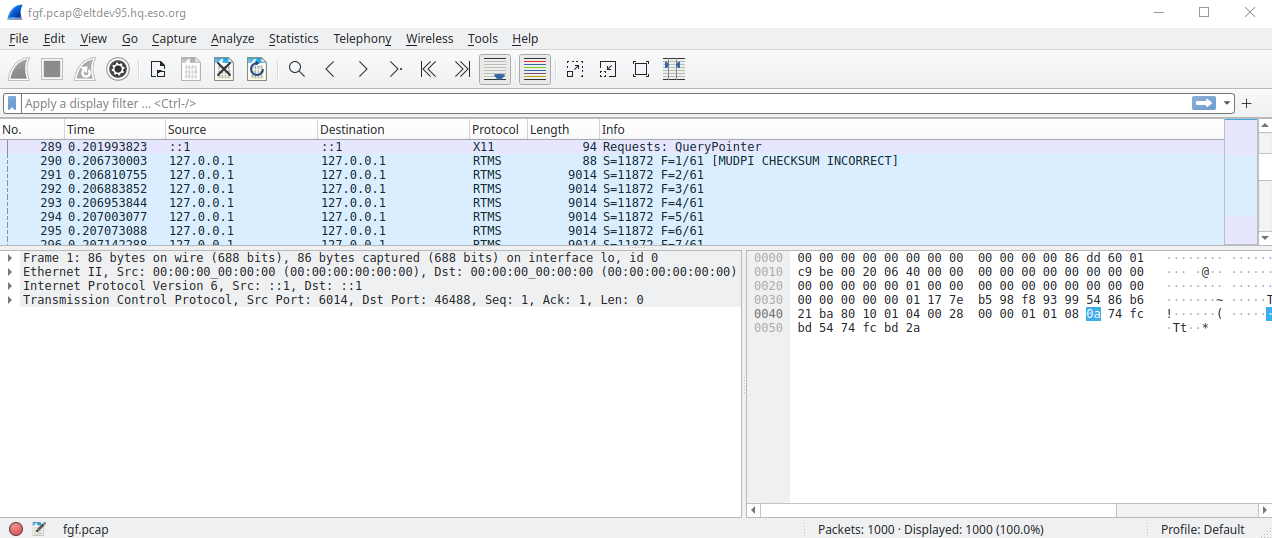
Now launch Wireshark on the captured network traffic data:

eltdev $ wireshark -r fgf.pcap -X lua_script:rtms.lua

If a message about the incorrect checksum is displayed, this is due to that the CRC checksum is not calculated and set in the FGF MUDPI packet creator.

In the screenshot can be seen how the RTMS Leader Packet (size=88) is received, followed by a series of RTMS Payload Packets of size 9014 (=Jumbo Packet). The last Payload Packet may be smaller (not shown). After the last Payload Packet, follows the RTMS Trailer Packet. Refer to the MUDPI/RTMS documentation for further information about these protocols.

Explaining in details how to use Wireshark to analyse the data, is not feasible here. Instead the user is kindly requested to seek further information about this from the Wireshark documentation and other public sources.

Other Tools & Means for Network Traffic Analysis

This section provides some information about how to analyse network traffic on a node, e.g. receiving RTMS data from a camera, which could be controlled by an FGF Application.

The proposed tests, are based on some basic commands, available on the ELT DevEnv platform.

This is useful to attempt to pinpoint issues.

It is not the intention to provide a complete guideline for using the various tools mentioned in this section. The purpose is merely to provide some input that can be used as starting point for getting acquainted with the tools and input for how to troubleshoot RTMS applications. For the proper documentation of the tools, refer to the appropriate documentation.

To analyse the volume of data going through an interface to ensure that it is consistent with the selected frame rate and size, the following command can be executed:

$ sar -n DEV 1 100

Note that even though the throughput seems to be correct, packet loss shall be analysed. Packets may be lost either in the Network interface (NIC) or because they could not be read by the application.

To monitor the traffic on the NIC, the tool named “ethtool” can be used in the following way:

$ watch -n 1 "ethtool -S <interface>"

Use “ip link show” or “ifconfig” to get information about network interfaces on the node. Example:

$ watch -n 1 "ethtool -S ens192"

The “ethtool” allows to inspect the current number of packets received as well, as packets with errors. Consult the documentation of “ethtool” for more information.

Another possibility to monitor a NIC is to use the command:

$ ip -s link show <address>

Example:

$ ip -s link show ens192

To monitor the traffic on a socket used by your application, run:

$ watch -n 1 "ss -u -a -m -O | grep <port>"

This generates an output of this kind (60000 being here the port number):

UNCONN 0 0 0.0.0.0:60000 0.0.0.0:* kmem:(r0,rb327680,t0,tb212992,f4096,w0,o0,bl0,d160300)

The significant piece of information is the last number, i.e. “d160300” that indicates the number of packets that could not be demultiplexed into the socket. In case of packet loss, the network stack behavior can be tuned via the following parameters (as root user):

Increase the maximum size of the socket receive buffer size on (rmem_max), e.g. “echo 16777216 > /proc/sys/net/core/rmem_max”.

Set the maximum number of packets that can be queued on the input side of a network interface, e.g: “sysctl -w net.core.netdev_max_backlog=4096”.

Default receive socket buffer size in bytes, e.g. “sysctl -w net.core.rmem_default=4000000”.

Set the maximum number of connections that can be queued for acceptance by a listening socket, e.g. “sysctl -w net.core.somaxconn=8192”.

Set the minimum socket receive buffer size for UDP: “sysctl -w net.ipv4.udp_wmem_min=16384”.