 mirror sites:
PL (internal link)
HQ
[?]
Quality Control and
Data Processing
UVES: ECH Flux calibration
The UVES pipeline delivers extracted spectra which are debiased, flattened, background subtracted, wavelength calibrated and extracted. If a master response curve exists (which depends on setting and epoch), the pipeline then does the final step, flux calibration. Otherwise it stops after the extraction. These extracted but uncalibrated data come in non-physical units ('quasi-ADU'), with their large-scale slope determined by the ratio of stellar and flat field spectral slopes. For line profile studies this is sufficient. If however an object has been observed in different setups and should ultimately be merged into one single result spectrum, it is very useful to have a correction for the instrument response slope.  Responses Curves
A standard star measurement is processed by the pipeline into the flat-fielded, extracted and wavelength-calibrated result, p_std. This pipeline product can be further processed (which includes extinction correction, normalization for exposure time, binning and gain) into the normalized standard star spectrum, f_std. This, divided into the tabulated flux, F_std, of the standard star, finally yields the response curve, R: R = F_std/f_std where F_std is in physical units (erg/[s cm**2 A]) and f_std is in quasi-ADU. Having determined a reasonable response curve R, it can readily be used to flux-calibrate any point-source object spectrum, f_obj:F_obj = f_obj*R. The precision of the flux calibration is limited by: All standard star measurements are processed by the UVES pipeline into response curves. These products (being delivered as UV_PRSP files) in principle measure the ratio (physical flux distribution/registered counts) per standard star but are not directly suitable for flux calibration. The typical output has very strong remnants of the flat-fielding process (order-scale ripples) and often a bad background subtraction (since data are typically taken in the twilight). Also the data have often very high signal and are poorly extracted by the optimum extraction routine. Furthermore the pipeline-delivered response curves lack Finally there is the fact that many standard stars have strong spectral features. Their spectra are compared to flux tables which have typically 50, or at best 16 A, resolution. Dividing the extracted spectra into the flux table values produces lots of 'quasi-emission' features which make their direct use for flux calibration impossible.
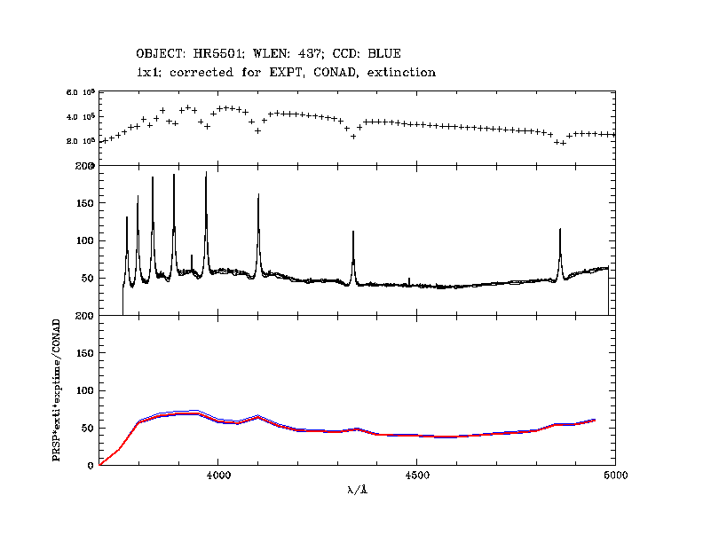
Above is an example which illustrates some of these problems with pipeline-processed response curves:
To overcome these problems and provide a set of UVES response curves useful for science flux calibration purposes, a set of properly selected input frames processed from STD star observations has been defined. Selection criteria were: These have been used to create master response curves which are binned to 50 A resolution. This avoids the quality problems of the high-resolution versions, and at the same time the problems of spectral features in the standard star data. The lower panel in the above figure shows the selected and corrected response curves for the setting 437BLUE (blue curves). The red curve is the averaged master response curve. The processing of the RED spectra was done with the flat-fielding method 'extract' which has no negative impact on the response curves since these are based on cursor-determined and tabulated value. There is however a scaling factor between the results with the 'extract' and those with the 'pixel' method. This scale factor (F) needs to be taken into account when a 'pixel' science spectrum is flux calibrated with an 'extract' master response curve. For the Blue Chip there is no such scale factor. The final master response curves have been edited in spectral regions with strong emission or absorption features. The underlying assumption is that the real instrument response varies only slowly over 50 A scales. They come per standard setting wavelength (346, 390, 437; 564, 580, 760, 860 REDL and REDU). No distinction is made between dichroics and non-dichroics.  Master Responses
To overcome these problems and provide a set of UVES response curves useful for science flux calibration purposes, a set of properly selected input frames processed from STD star observations has been defined. Selection criteria were: These have been used to create master response curves which are binned to 50 A resolution. This avoids the quality problems of the high-resolution versions, and at the same time the problems of spectral features in the standard star data. The lower panel in the above figure shows the selected and corrected response curves for the setting 437BLUE (blue curves). The red curve is the averaged master response curve. The processing of the RED spectra was done with the flat-fielding method 'extract' which has no negative impact on the response curves since these are based on cursor-determined and tabulated value. There is however a scaling factor between the results with the 'extract' and those with the 'pixel' method. This scale factor (F) needs to be taken into account when a 'pixel' science spectrum is flux calibrated with an 'extract' master response curve. For the Blue Chip there is no such scale factor. The final master response curves have been edited in spectral regions with strong emission or absorption features. The underlying assumption is that the real instrument response varies only slowly over 50 A scales. They come per standard setting wavelength (346, 390, 437; 564, 580, 760, 860 REDL and REDU). No distinction is made between dichroics and non-dichroics. You can download and view master reponses here  How to
How to flux calibrate the data If fed with the proper master response curve, the UVES pipeline will generate flux-calibrated spectra as final output. As mentioned above, one has to be apply a scaling factor (F) when a 'pixel' science spectrum is flux calibrated with an 'extract' master response curve for the 760 and 860 spectra. The science spectrum has to be multiplied by F.
If no master response curve is provided, the pipeline will stop one step before and deliver reduced (but not flux-calibrated) spectra.
The product fluxed_science comes in physical units [10**(-16) erg/s/cm**2/A] vs. A.  Testing the Flux calib
How to test the flux calibration
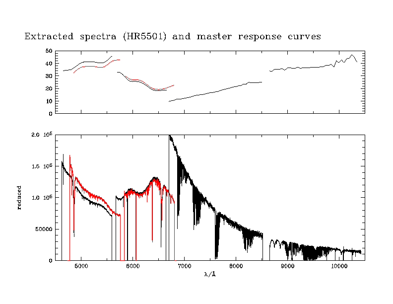
As a check for this procedure, we have selected spectra of a flux standard star, HR5501. These data have been measured in all standard settings in the same night (2002-02-09). For the purpose of this test, they have been processed by the pipeline as SCIENCE spectra. The following figure shows the pipeline-delivered extracted flux (red settings 564/580/860 REDL and REDU CCDs) and the master response curves (top) for these settings. Setting 580 is plotted red, the others in black.
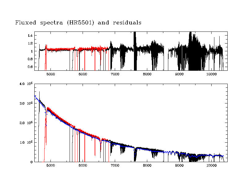
In the next figure, we see the flux calibrated spectra, i.e. the product of the extracted spectra and the master response curves. These spectra have physical units (10e-16 erg/s/cm**2/A). The tabulated fluxes, in the same units, are overplotted as blue dots. The upper panel has the residual fluxes (measured divided by tabulated). These never exceed 10% in continuum regions. Strong line features of course produce larger deviations. The systematic shifts come from differences between the master response curve used here (derived as average from several different input curves), and the individual response curves for HR5501.
In conclusion, (i) the master response curves can be reasonably precisely constructed from day-to-day response curves, with the corrections described; (ii) these master response curves can be used in a straightforward way to flux-calibrate the science spectra.
|
||||||||||||||||||||||
| |
||||||||||||||||||||||
 |
|
|||||||||||||||||||||


