
Description of the reduction of the SOFI polarimetric data (by Nancy Ageorges)
Purpose of this exercise:
Calibrate the instrument in terms of instrumental polarization.
General information:
To achieve polarimetric observations with SOFI a Wollaston prism and an adequate special mask are installed along the light path. The image frame is thus split horizontally into 6 bands corresponding (from top to bottom) to a sky (E and O vectors), the object (E and O vectors) and another sky (again E & O vectors). The data format is very well explained by J. Walsh, who derived the instrumental polarization of this instrument from observations taken in 1997.
Flatfields:
Faltfield data have been acquired with the light on & off at different position angles, that should correspond to the sky position angles used during the observations, i.e. 0, +22.5, +45, +67.5, +90, +180 degrees.
The purpose of subtracting the 'off' from the 'on' images is to get rid of all noise contribution (darks, ...) and be left with only the flatfield contribution.
All 'on' positions did not have a corresponding 'off' position. '0', '+45' and '+90' have their own on-off frames. For PA = -22.5, the off-frames of '-45' degrees have been used. The 'off-frames' taken with an angle of '+90' have been used for on-frames taken at +67 and +180 degrees. No flatfield has been acquired at position +22.5, but at -22.5.
Looking at the different dome flatfield, it has been noticed that they are polarised (of the order of 2%), because of the way they have been acquired: the source of light comes from an angle that is different from the angle at which the telescope is looking at the flatfield screen. See Fig. 1, to understand.
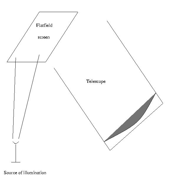
Figure 1: Description of the set-up for flatfield acquisition
The polarisation of the flatfield data is 'artificial' and not related to either the instrumental or the sky polarisation. Correcting with such flatfields would have meant introducing an extra polarization. It has therefore been decided to average these flatfields to obtain a 'non-polarised' average flatfield to correct the data. The absence of one of the polarisation angles introduce however a small error (<~1%).
Alternative ways of doing flatfield:
1/ rotate the polarizer in front of the instrument to average out any polarisation dependence.
This is not feasible at the NTT, since the rotation of the polariser is assured by the telescope rotator. The Wollaston itself has a fixed orientation compared to the detector.
2/ illuminate the detector directly rather than with a reflecting screen.
This would mean sky flats. The amount of flats we did, did not allow for that solution (lake of time).
Note that the CCD pixel-to-pixel flatfield is independent of the polarization. This is however not the case of the field illumination.
Data reduction:
For most data, reduction has been done with and without flatfielding the data, in order to be able to estimate the effect of the flatfield correction on the data (the polarization changes by 1 to 2%).
Since for each angle, data have been taken at three different positions on the CCD (Fig. 2), this has been used to determine the sky contribution. Sky frames have been created in two different ways:
1/ the min of the three frames has been taken. This method under-estimates the exact sky contribution but has the advantage to avoid 'source' overlap in crowded fields.
2/ For one position the mean of the two other positions has been taken as a sky.
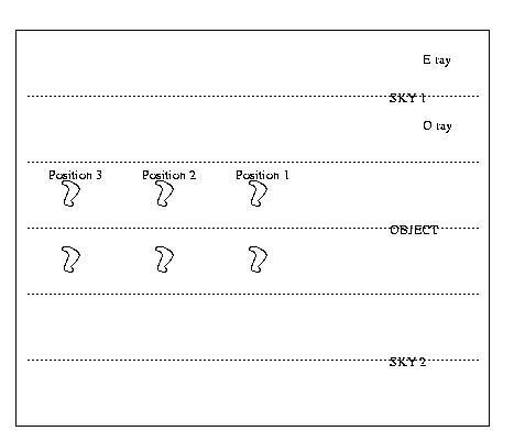
Figure 2: Scheme of the data format,
The results obtained with both methods have been compared. The results are identical to less than 1%. For each calibration source, the flux of the star has been calculated, in ADUs, adding the pixel value within a circle of given radius (6 to 10 pixels depending on the seeing), for each position angle and each polarization 'E' or 'O'. The results have been plotted as a function of the position angle at which they have been acquired. Since the polarization is a cosine function of period $\pi$, values acquired in 'E' at 0 degrees should correspond (within the photometric stability) to values obtained in 'O' at 90 degrees.
Doing this, we noticed a 'huge' jump in intensities between values derived from 'E' and 'O' fields. After checking that no mistake has been done during the analysis of the data, the only logical conclusion was that the Wollaston does not transmit the same way, i.e. with the same efficiency, in the 'E' and 'O' band. It is thus necessary to correct for this effect.
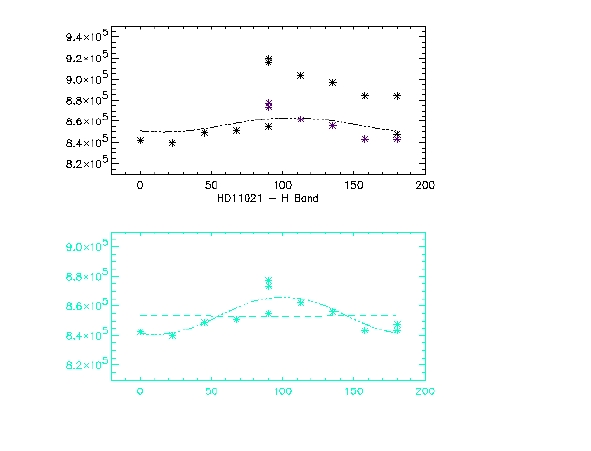
Figure 3: Example of data. Plots of intensity versus polariser position angle. Top panel: raw data (black) and corrected ones (purple) after application of the factor ~1.04. Lower panel, resulting data from which the instrumental polarisation has been derived ('cos(2$\theta$)'fit over plotted). The dispersion of points at 0 and 90 deg. corresponds to the photometric variation.
Two methods, detailed hereafter have been used. The ultimate aim is to determine the degree of instrumental polarisation and see if there is any correlation between the angle of instrumental polarisation and the paralactic angle at which data have been acquired, as is expected for a Nasmyth telescope like the NTT.
Method 1: (Automatic fitting)
A 'cos(2$\theta$)' has been fitted through the first half of the data ('O' data corresponding to angles between 0 and 90 degrees). We then fitted the results to the second half of the curve and calculated a mean ratio difference. This second half data set ('E' data between 90 and 180 degrees) has then been divided by this factor. Afterwards a new 'cos(2$\theta$)' function has been fitted to all the data (original first half + modified second half), which give us the final instrumental P and $\theta$. This has been achieved thanks to an IDL procedure.
Method 2: (Eye adjustment)
The ratio between the first half of the sinusoid and the second has been estimated by eye to give a 'smooth' sinusoid. From the values obtained for different filters and different sources, an average correction factor of 1.06 in J & H and 1.04 in K has been used to correct the data intensity. Then a cosine curve has been fitted (in MIDAS).
Note: Previously the IDL and MIDAS procedures have been tested on the 'raw' data and have been found to give the same result within 0.1\% and 0.5$^{\circ}$, which corresponds to the calculation accuracy fixed in the autromatic fitting procedure.
Results:
| J | H | K | ||||
| P(%) | Angle (deg) | P(%) | Angle (deg) | P(%) | Angle (deg) | |
| Unpolarised Sources | ||||||
| HD 11021 | 1.9 | 160.5 | 1.5 | 159 | 1.3 | 177.5 |
| 1.64+/-.26 | 4.84+/-12.8 | 1.21+/-.28 | 4.96+/-23.6 | 1.23+/-.22 | .44+/-17.5 | |
| HD 195455 | 1.9 | 134 | 1.7 | 128 | 1.1 | 139 |
| 1.63+/-.32 | 143.7+/-11.8 | 1.32+/-.22 | 144+/-10 | 1.32+/-.29 | 129.9+/-12.9 | |
| HD 222126 | 2.1 | 42 | 1.9 | 52 | 1.2 | 43 |
| 1.56+/-.34 | 13.5+/-15.4 | 1.19+/-.36 | 9.46+/-21 | .58+/-.4 | 160+/-47 | |
| Polarised Sources | ||||||
| HD 150913 | 2.8 | 180 | 1.6 | 180 | 1.9 | 180 |
| 3.51+/-.45 | 37.+/-7.9 | 2.42+/-.12 | 29.15+/-2 | 2.06+/-.2 | 27.7+/-6.8 |
Table 1: Determined SOFI+NTT instrumental polarisation. Values on the same level as the name of the source, have been determined with Method 1; the lower values results from MIDAS (Method 2).
The results, of the automatic fitting procedure, have shown to give a value close to 1.04, for all wavelengths, for the correction factor to apply. The results of this procedure are given with an error of 0.1% and 0.5$^{\circ}$. The'eye' fit for HD222126 is poor. It gives much better results if no correction factor is applied to the original data! For HD150193, the position angle is poorly determined by the automatic fitting; in this case the error bar is clearly larger than 0.5$^{\circ}$ but not exactly determined.
Globally, except for the two cases mentioned above, where either of the two methods gives a poor fit, the results can be considered as equivalent within the error bars.
| Source | Paralactic | Angle |
| Range of values | 'Mean' value | |
| HD 11021 | [-95,-90] | -92.5 |
| HD 195455 | [107.1,107.6] | 107.5 |
| HD 222126 | [-150,138] | 174 |
| HD 150193 | [107.4,108] | 107.7 |
Table 2: Values of the paralactic angle during the observation.
The next logical step was to plot the position angles determined versus the averaged parallatic angle at which data have been acquired. This is represented Fig. 4, which a representation in the (U,V) plane.
No clear tendency can be found, and that is where our understanding stops. Do we have two components? A constant component and one dependent on the parallactic angle?
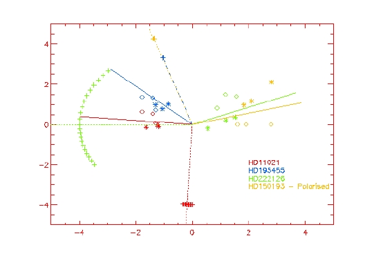
Figure 4: Plot of the instrumental polarization versus the paralactic angle. The stars are the resultsof the automatic fitting, and diamonds come from the 'eye adjustment' technique. Information are color coded per source. The '+' are the corresponding paralactic angles. Full lines are indicative of the averaged instrumental polarisation angle for a source. The corresponding direction of the paralactic angle is represented by a dotted line.