This tutorial provides a step-by-step example of the preparation of a set of Observing Blocks (OBs) with VISIR, the VLT spectrometer and imager for the mid-infrared. The specifics of this tutorial pertain to the preparation of OBs from Period 102 onwards.

To follow this tutorial you should have familiarity with p2 : the web-based tool for the preparation of Phase 2 materials.  Please refer to the main p2 webpage (and the items in the menu bar on the left of that page) for a general overview of p2 and generic instructions on the preparation of Observing Blocks (OB).  Screenshots for this tutorial were made using the demo mode of p2, but should not differ in any way from one's experience in preparing your own OBs under your run.

0: Goal of the Run

In this tutorial we will prepare two OBs, one imaging OB and one spectroscopic OB. In both cases the target is a young stellar object named He3-298 possessing a circumstellar disk. We assume that you wish to image He3-298 with a PAH filter at 11.25 micron and observe it spectroscopically at low resolution. The target has the following coordinates: RA(2000) = 09 36 44.4, Dec(2000) = -53 28 00. We will start with the construction of the imaging OB, followed by a long-slit spectroscopy OB.

The sample OBs will illustrate the use of a variety of features of p2 and illustrate the kind of decisions to be taken at the time of preparing in advance an observing run, as well as some aspects that are specific to the preparation of OBs for VISIR.

1: Getting started

The Phase 2 process begins when you receive an email from the ESO Observing Programmes Office (OPO) informing you that the allocation of time for the coming period has been finalized and that you can view the results by logging into the User Portal and clicking on "Check the time allocation information" (within the Phase 1 card). Note that the username and password that you need to use for the User Portal are the same as those you will use to prepare your OBs.

You follow the instructions given by ESO and find that time was allocated to your run with VISIR. Therefore, you decide to start preparing your Phase 2 material. First, you collect all the necessary documentation:

• The VISIR User Manual
• The VLT Service Mode Guidelines
• The p2 Documentation referred to above.

to the top

2: Your first OB - Starting with p2

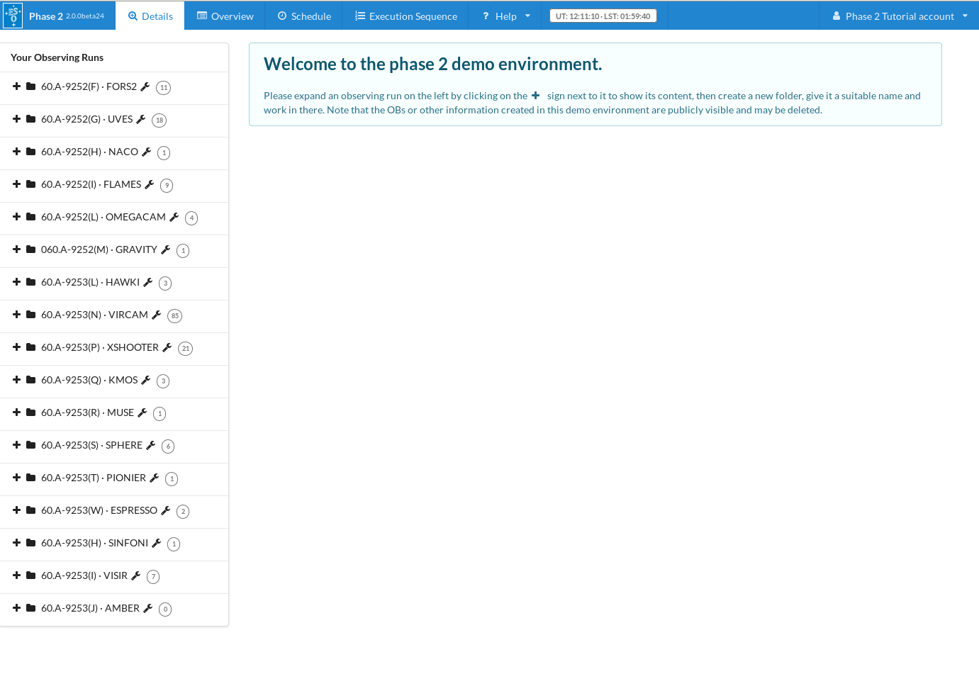
Runs for a number of instruments appear in the lefthand column, since the p2 demo facility is used for all of them.  Similarly, if you log into p2 (instead of p2demo) with your own ESO User Portal credentials, you will get the list of all the runs for which you are PI, or for which you have been declared as a Phase 2 delegate by one of your colleagues.

Select the folder corresponding to the VISIR tutorial run, 60.A-9253(I) by clicking on the + icon next to it.  In this tutorial we assume that time was allocated in Service Mode.  This is indicated by the small wrench icon that appears next to the RunID.  "Inside the run" you will see (at least) one folder, called "VISIR Tutorial".  That folder contains the final product of the tutorial you are now reading.  You can refer to the contents of that folder at any time, perhaps to compare against your own work.

You can now start defining your observations.  In the p2 demo you must first start by creating a folder, within which you will put your own content.  Because the p2 demo is online and accessible to anyone you may see folders belonging to other people here, though after-the-fact cleanup is encouraged and possible. 

to the top

2.1: Define an imaging OB with p2

Once you have selected the VISIR folder, you can start defining your first OB.

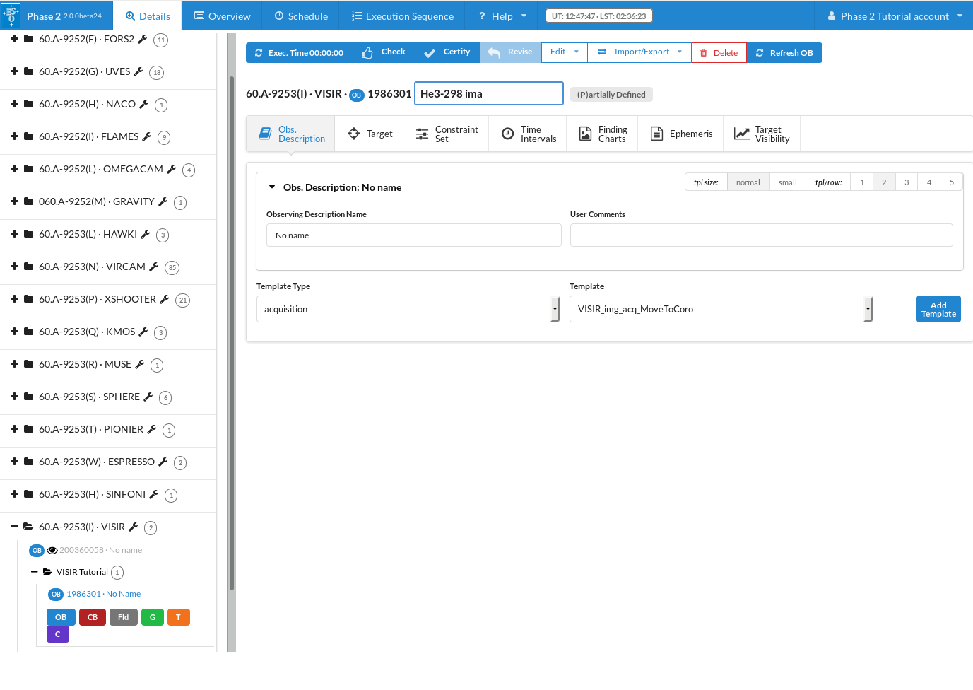
First, click on the OB icon within the newly created folder. This will create an empty new OB. You may now change the name of the newly created OB. Preferably, you like to be able to identify later that this OB is associated with the target He3-298 and that it is an imaging OB. Therefore, you choose the OB name He3-298-ima. Click on the "No Name" OB name listed within the OB contents, then type this name He3-298-ima.

The OB contents should now appear as this:

to the top

2.1.1: Filling in the Basic Information

Obs. Description Name

It may be useful in many cases to have an easy way of identifying an Observing Description, like when having observations of a number of targets performed with identical instrument configuration and observation template parameters. The Observation Description Name field allows you to define names for the Obseration Descriptions. In this tutorial OB the observation description will define the use of the PAH2 filter at 11.25 micron. Thus, we enter the name Imaging_PAH2 in the Observation Description Name field.

User Comments

For VISIR, it is compulsory to list the exepected brightness of the target (in mJy) in the User Comments field of the OB. In addition, the User Comments field can be used for any information you think is important for the night astronomer at the time the OB is executed, e.g. to keep further track of the characteristics of the OB, to alert the staff on Paranal to special requirements (but also see the reference below to the Calibration Requirements field).

to the top

2.1.2: Defining the acquisition template

The first template that must be part of any science OB is the acquisition template, so let us define it next. In the Template Type list, make sure that the acquisition entry is highlighted. This will list all the acquisition templates available for VISIR in the Template list next to it.

After reading the description of the templates in the User Manual, you have noticed that the VISIR_ima_acq_MoveToPixel template is your choice, because you are using the intermediate pixel scale (pfov 0.076 arcsec) and you want to make sure that your target gets very well centered. You thus click on this template in the Template list, and then on the Add Template button next to it. The p2 window should now look like this:

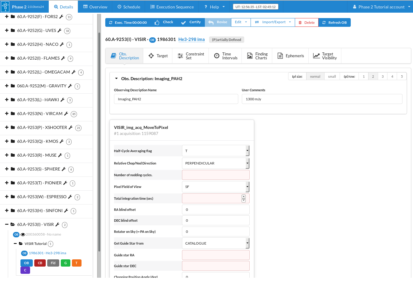
Now, you need to decide on the acquisition parameters, and if necessary, modify the default values given in the acquisition template.

There are three parameters related to the telescope nodding and the secondary mirror chopping. Since your target is relatively little extended (less than 4 arcseconds in diameter) and also an isolated source, you decide to chop on the array, without changing the default chopping position angle. Furthermore, since you will choose a perpendicular relative chop/nod direction in your later science observations, you also select a perpendicular relative chop/nod direction for the acquisition. Thus, you enter the parameters (or select from the drop-down menu):

• Relative Chop/Nod Direction: PERPENDICULAR
• Chopping Position Angle: 0 (Default value)
• Chopping Amplitude: 10

The next parameter to enter is the total integration time that will be necessary to clearly identify your target. Since He3-298 is bright, the minimum of 30 seconds is sufficient for that purpose. Hence, you enter

• Total integration time: 30.0
• Number of nodding cycles: 1

You will also have to make a choice on the filter used during the acquisition, which should, in general, be selected in such a way that a high signal to noise on the target is achieved in relatively short time. In our tutorial example the continuum filter next to the PAH2 filter is the right choice. Furthermore, you wish to use the finest pixel scale. Therefore, you select from the drop-down menus:

• Imager filter: PAH2_2
• Pixel Field of View: SF
  

For the rest of the parameters in the acquisition template you can leave the default values.

to the top

2.1.3: Inserting Target Information

Now press the Target tab at the top of the edit window. The target edit window appears with fields in which to insert your target name, coordinates and proper motion. Coordinates and proper motions can either be manually inserted, or be retrieved from the SIMBAD database by pressing the "resolve" button after entering the target name.

We now enter the target name, which can be (for easy cross-identification purposes) the same name as used in the OB naming, in other words, insert

• Name: Hen 3-298

And we press the "resolve" button to automatically fill out the right ascension, declination and proper motion of our target.

The acquisition template including the target information is now complete, and the window should look like this:

to the top

2.1.4: Setting the Constraint Set

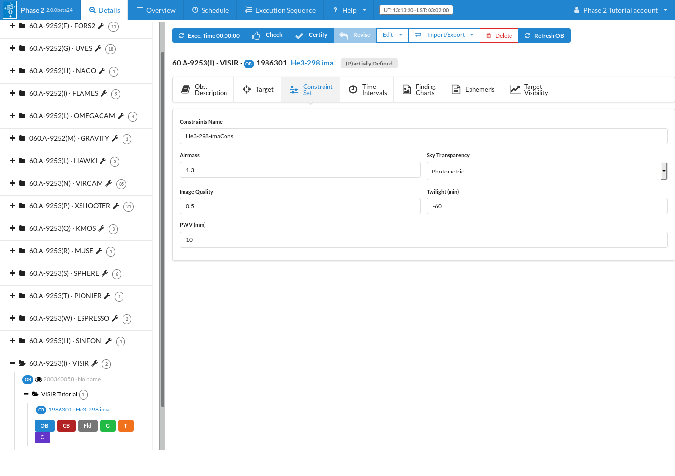
As stated in Section 1, we assume for the purposes of this tutorial that the program has been allocated time in Service Mode. You thus need to specify a set of constraints, which indicate under which conditions your OB can be executed.You can do this by clicking on the Constraint Set icon at the top of the edit window and filling the entries under it:

Name:

First, give a descriptive name to the constraint set about to be defined. Since you have decided that this constraint set will be applied to all the imaging OBs of this target, you type He3-298-imaCons in the Name field.

Sky transparency:

Since we assume that your imaging observations aim at constraining as accurate as possible the mid-infrared luminosity of He3-298 and itscircumstellar disk, you need very good atmospheric conditions. You request Photometric conditions in the Sky Transparency entry.

Image Quality:

As for the image quality constraint, you know that the image quality at 10 microns is diffraction-limited if the optical seeing is better than ~0.8 arcsec (which is the constraint you entered at Phase 1). Since spatial resolution is a key issue for your study, you enter 0.5 (corresponding to the expected image quality in the PAH2 filter we will be observing with) in the image quality field.

Airmass:

The airmass is not a stringent parameter for the imaging part of your programme, you thus enter 2.0 in the Airmass field.

Lunar Illumination and Moon Angular Distance

The moon has essentially no effect at all on the VISIR data quality, and constraints related to the moon are not considered for OB qualification.

Twilight Constraint:

Since the solar position has little effect on the sky brightness in the mid-infrared, you are Ok with your observations being doing in twilight. Therefore you enter -60 in the Twilight field to allow your observations to be started a maximum of 60 minutes before the start of astronomical twilight.

PWV:

As you are doing imaging observations in the N-band, precitable water vapour (PWV) is only moderately important for your science goals, so you request your observations to be done under PWV conditions of 10 mm or less. Therefore you enter 10 in the PWV field.

Note that in your Phase 1 proposal you already specified some of these constraints (sky transparency, seeing). You must make sure that none of the constraints specified in Phase 2 is more stringent than the corresponding one specified at Phase 1.

to the top

2.1.5: Setting the time intervals

We will assume now that your VISIR observations are part of a larger multi-wavelength project and that the VISIR observations should be carried out simultaneously with some satelite observations that are performed between October 01-31 2018. You can specify this, i.e. the execution of your VISIR OB between October 01 and October 31, 2018 under the Time Intervals tab:

• Press Add to add a single time interval.
  
• Modify the lower boundary (the left-hand side entry) of the time interval to the specified starting date of your time window, keeping the same format. In the present case, the entry should read 2018-10-01T00:00:00.
• In the same way, modify the upper boundary of the time interval to 2018-10-31T00:00:00.

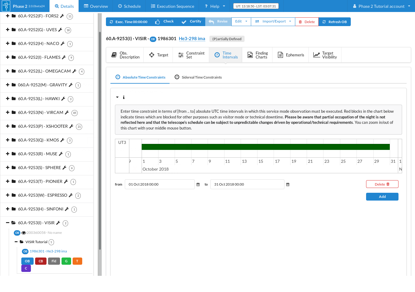
If your observation could be executed in other, non-contiguous time windows, you could define several intervals in the same way as described. However, setting restrictive time intervals for an OB, and thus narrowing the possible execution times/dates, will limit the possibility that your OB will be successfully executed during the observing period. It thus should only be used when strictly necessary.

to the top

2.1.6: Defining the Observation Description

Once the acquisition and the items Target,  Constraint Set, and Time Intervals are completed, the science template(s) can be inserted. Click on Obs. Desciption to view the observation description.

On Template Type, select now science. The existing VISIR science templates will appear. Select the template VISIR_img_obs_AutoChopNod and click on Add Template. The template will be attached to the grid below next to the acquisition template selected and filled previously.

Several parameters have to be defined for this template. In the following we discuss each of them and justify a certain choice based on the properties of the target He3-298 and the scienctific goal of this imaging OB. First, you have to decide if you prefer to nod perpendicular or parallel to the direction of the chop. From the manual you extract that for not very extended sources and observations that aim at high spatial resolution, the perpendicular relative chop/nod is recommended. From the pull-down menu you therefore select:

• Relative Chop/Nod Direction: PERPENDICULAR

Several bad pixels or cosmics will produce an errornous response at some parts of the array. Therefore you want to avoid the target's signal falling permanently on a bad pixel and you choose to jitter on the nod positions by setting:

• Random Jitter Box Width: 3

After using the exposure time calculator for VISIR in imaging mode, you know that 600 sec of total integration time is needed on He3-298 in order to reach the signal to noise ratio you want. We will divide this into 3 nodding cycles to get good sky subtraction. Thus,

• Total integration time: 600
• Number of nodding cycles: 3

The next two parameters, again, are related to chopping and we will make the same selection as in the acquisition template, because the same rules apply here:

• Chopping Position Angle: 0 (default)
• Chopping Amplitude: 10

Then, you have to select the imaging filter for this observation. In principle, you are interested in imaging the PAH feature at 11.25 microns, which implies the filter PAH2. But of course, it is also necessary to perform the same observations with a reference filter, close by in wavelength and centered on the continuum in orderto separate the continuum contribution from the true 11.25 micron emission. Since the continuum reference filter PAH2_2 is already in place (being used for the acquisition), we do the continuum imaging first and select:

• Imager filter: PAH2_2
• Pixel Field of View: SF

If you followed all the indications given so far, the View OB window should look like this now.

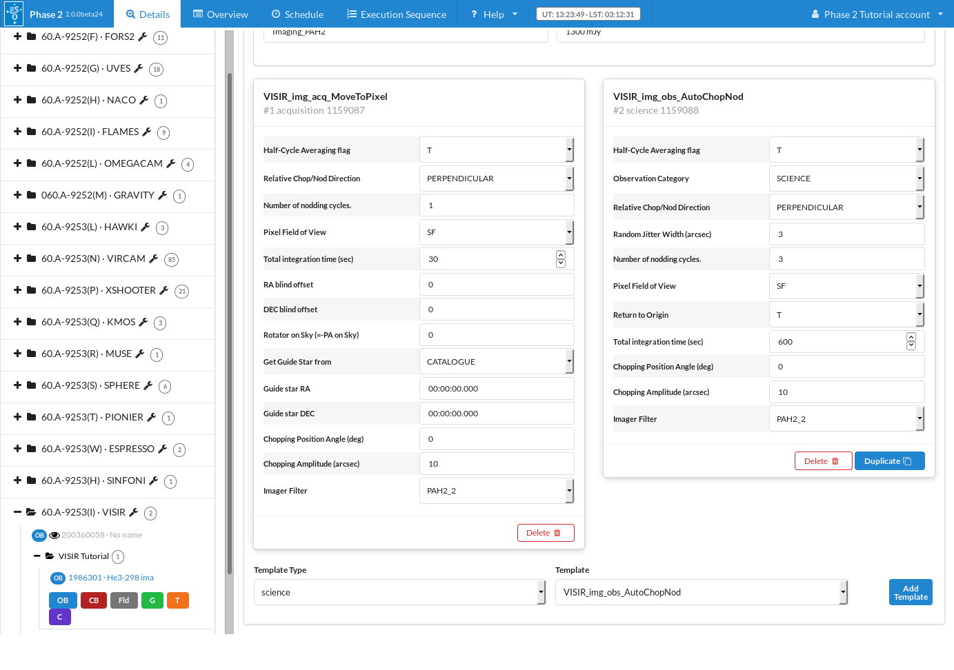
The observation that must now follow, and which should be defined within the same OB, is the imaging at the actual PAH filter, PAH2. In other words, you must append another VISIR_img_obs_AutoChopNod template. We could select the template from the list of science templates and again fill out all parameters, but in this case it may be easier to copy the existing VISIR_img_obs_AutoChopNod template, since it already has many of the parameters we want filled out. So we simply press "Duplicate" in the exisiting VISIR_img_obs_AutoChopNod template, and all we have to do is change the imaging filter:

• Imager filter: PAH2

The p2 window should now look like this:

The only other thing that you should really do at this point is to check the execution time for this OB. Click on the Exec. Time tab at the top of the screen to re-calculate the execution time for your OB.

to the top

2.1.7:Attaching Finding Charts

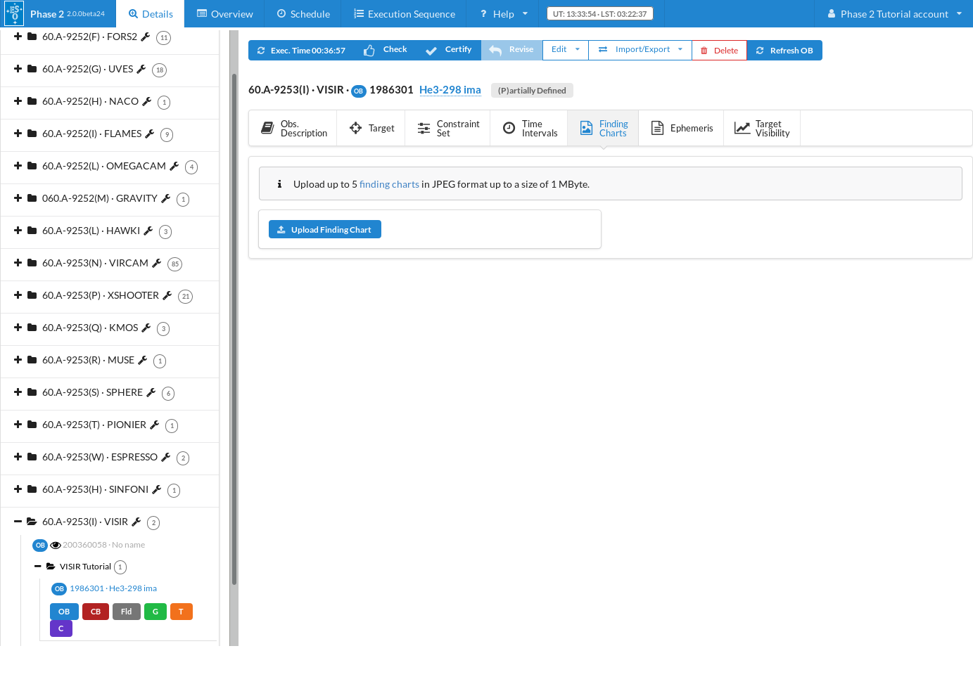
The last thing to do, which finishes the preparation of a single OB, is to attach the respective Finding Chart(s) to the OB. The Finding Charts must be prepared as jpeg-files and must fulfill all general and VISIR-specific requirements for finding charts. You can use any tool of your choice to create the Finding Charts in jpeg-format. p2, however, does not contain such an option.

Let's assume you have prepared a jpeg-Finding Chart for this tutorial run [remember:run ID 60.A-9253(I)], which you called 60.A-9253I.he3-298.jpg, and which is saved in a sub-directory of your home directory.

Now, in the p2 main window clickon the "Finding Charts" tab, and select the finding chart(s) which should be attached to the OB:

to the top

2.2: Define a spectroscopic OB with p2

In the next section of this tutorial, we will define an OB to do long-slit low-resolution spectroscopy on the same target, He3-298.

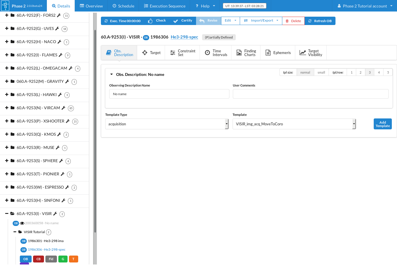
We start by again OB icon in our VISIR tutorial folder to create a new OB. You may now change the name of the newly created OB. Preferably, you like to be able to identify later that this OB is associated with the target He3-298 and that it is a spectroscopic OB. Therefore, you choose the OB name He3-298-spec. Click on the OB, and press enter, then type this name He3-298-spec.

The OB contents should now appear as:

to the top

2.2.1: Filling in the Basic Information

Obs. Description Name

It may be useful in many cases to have an easy way of identifying an Observation Description, like when having observations of a number of targets performed with identical instrument configuration and observation template parameters. The Obs. Description Name field in the View OB window allows you to define namesf or the Observations Descriptions. In this tutorial OB the observation description will define the use of low-resolution spectroscopy across the N-band. Thus, we enter the name Spectroscopy-N in the Obs. Description Name field

User Comments

For VISIR, it is compulsory to list the exepected brightness of the target (in mJy) in the User Comments field of the OB. In addition, the User Comments field can be used for any information you think is important for the night astronomer at the time the OB is executed, e.g. to keep further track of the characteristics of the OB, to alert the staff on Paranal to special requirements (but also see the reference below to the Calibration Requirements field).

to the top

2.2.2: Defining the acquisition template

The first template that must be part of any science OB is the acquisition template, so let us define it next. In the TemplateType list, make sure that the acquisition entry is highlighted. This will list all the acquisition templates available for VISIR in the Template list next to it.

After reading the description of the templates in the User Manual, you have noticed that the VISIR_spec_acq_MoveToSlit template is your choice, because you are doing spectroscopy of a relatively bright source. You thus click on this template in the Template list, and then on the Add Template button next to it. The window should now look like this:

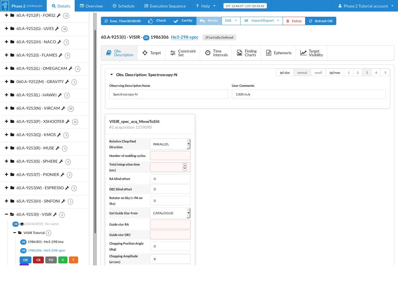
Now, you need to decide on the acquisition parameters, and, if necessary, modify the default values given in the acquisition template.

There are three parameters related to the telescope nodding and the secondary mirror chopping. Since your target is relatively little extended (less than 4 arcseconds in diameter) and also an isolated source, you decide to chop on the array. However, your source has a companion at a position angle of 64 degrees, which you would like to avoid having in the slit. So you choose a slit rotator angle of 360-154=206 degrees, which is perpendicular to this, and a relatively narrow slit width of 0.4 arcseconds. Furthermore, since you wish to chop within the slit, you choose a long slit, a chopping angle that is identical to the slit rotator angle, and a parallel relative chop/nod direction. Thus, you enter the parameters (or select from the drop-down menu):

• Relative Chop/Nod Direction: PARALLEL (Default value)
• Rotator on Sky (=-PA on Sky): 206
• Chopping Position Angle: 206
• Chopping Amplitude: 10
• Spectrometer Slit Type: LONG (Default value)
• Spectrometer Slit Width: 0.40

The next parameter to enter is the total integration timethat will be necessary to clearly identify your target. Since He3-298 is bright, 60 seconds is sufficient for that purpose.Hence, you enter

• Total integration time: 60.0

You will also have to make a choice on the filter used during the acquisition, which should, in general, be selected in such a way that a high signal to noise on the target is achieved in relatively short time. Since our target He3-298 has a relatively red energy distribution over the N-band, we choose the long-wavelength broad-band N_LW filter. Therefore, you select from the drop-down menus:

• Acquisition filter: ARIII

For the rest of the parameters in the acquisition template you can leave the default value.

to the top

2.2.3: Inserting Target Information

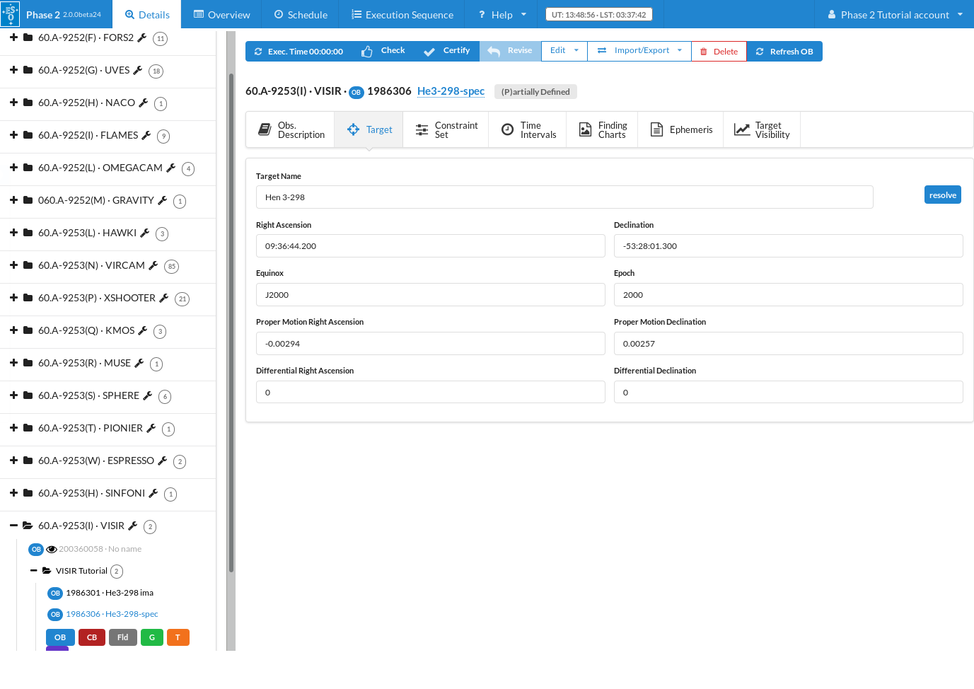
Now press the Target tab at the top of the edit window. The target edit window appears with fields in which to insert your target name, coordinates and proper motion. Coordinates and proper motions can either be manually inserted, or be retrieved from the SIMBAD database by pressing the "resolve" button after entering the target name.

We now enter the target name, which can be (for easy cross-identification purposes) the same name as used in the OB naming, in other words, insert

• Name: Hen 3-298

And we press the "resolve" button to automatically fill out the right ascension, declination and proper motion of our target.

The acquisition template including the target information is now complete, and the window should look like this:

to the top

2.2.4: Setting the Constraint Set

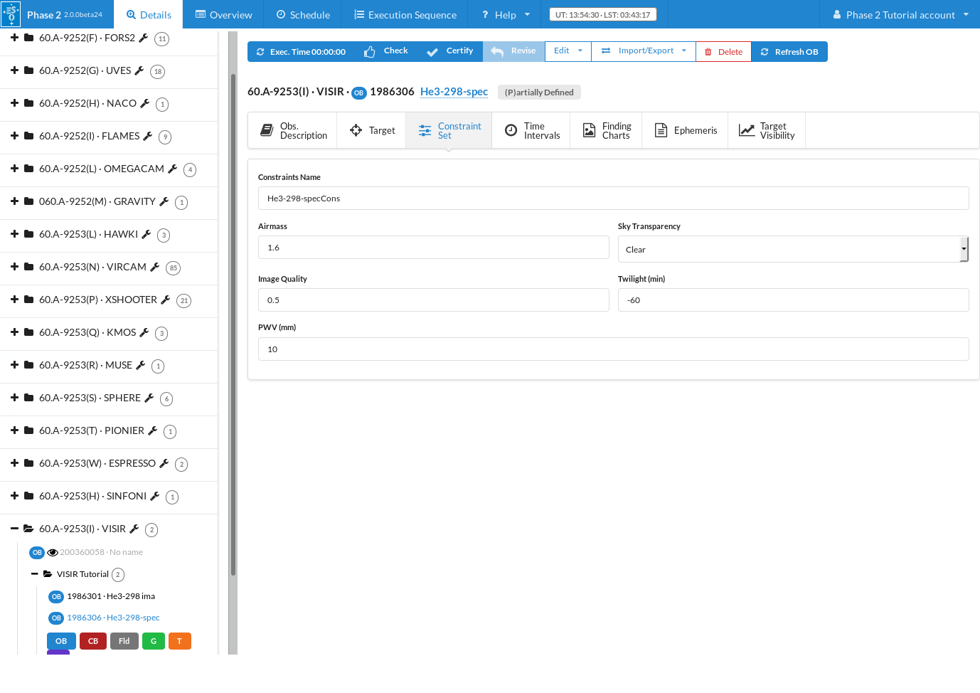
As stated in Section 1, we assume for the purposes of this tutorial that the program has been allocated time in Service Mode. You thus need to specify a set of constraints, which indicate under which conditions your OB can be executed.You can do this by clicking on the Constraint Set icon at the top of the edit window and filling the entries under it:

Name:

First, give a descriptive name to the constraint set about to be defined. Since you have decided that this constraint set will be applied to all the spectroscopic OBs of this target, you type He3-298-specCons in the Name field.

Sky transparency:

You wish to obtain your spectroscopic observations of He3-298 in conditions offering good atmospheric transparancy in the direction of your target. You thus request Clear conditions in the Sky Transparency entry.

Image Quality:

As for the image quality constraint, you know that the image quality at 10 microns is diffraction-limited if the optical seeing is better than ~0.8 arcsec (which is the constraint you entered at Phase 1). Since spatial resolution is a key issue for your study, you enter 0.5 (corresponding to the expected image quality in the PAH2 filter we will be observing with) in the image quality field.

Airmass:

To achieve a good telluric correction, you wish your observations to be done at relatively low airmass. You thus enter 1.6 in the Airmass field.

Lunar Illumination and Moon Angular Distance

The moon has essentially no effect at all on the VISIR data quality, and constraints related to the moon are not considered for OB qualification.

Twilight Constraint:

Since the solar position has little effect on the sky brightness in the mid-infrared, you are Ok with your observations being doing in twilight. Therefore you enter -60 in the Twilight field to allow your observations to be started a maximum of 60 minutes before the start of astronomical twilight.

PWV:

As you are doing observations in the N-band, precitable water vapour (PWV) is only moderately important for your science goals, so you request your observations to be done under PWV conditions of 10 mm or less. Therefore you enter 10 in the PWV field.

Note that in your Phase 1 proposal you already specified some of these constraints (sky transparency, seeing). You must make sure that none of the constraints specified in Phase 2 is more stringent than the corresponding one specified at Phase 1.

to the top

2.2.5: Setting the time intervals

We will assume now that your VISIR observations are part of a larger multi-wavelength project and that the VISIR observations should be carried out simultaneously with some satelite observations that are performed between October 01-31 2018. You can specify this, i.e. the execution of your VISIR OB between October 01 and October 31, 2018 under the Time Intervals tab:

• Press Add to add a single time interval.
  
• Modify the lower boundary (the left-hand side entry) of the time interval to the specified starting date of your time window, keeping the same format. In the present case, the entry should read 2018-10-01T00:00:00.
• In the same way, modify the upper boundary of the time interval to 2018-10-31T00:00:00.

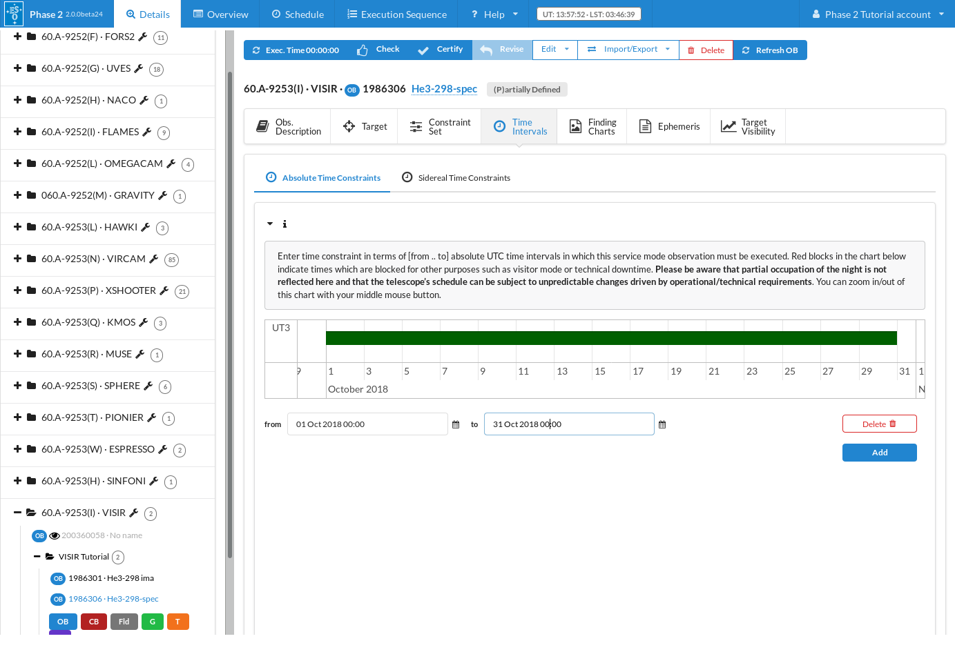
If your observation could be executed in other, non-contiguous time windows, you could define several intervals in the same way as described. However, setting restrictive time intervals for an OB, and thus narrowing the possible execution times/dates, will limit the possibility that your OB will be successfully executed during the observing period. It thus should only be used when strictly necessary.

to the top

2.2.6: Defining the Observation Description

Once the acquisition and the tabbed items Target, Constraint Set, and Time Intervals  are completed, the science template(s)can be inserted.

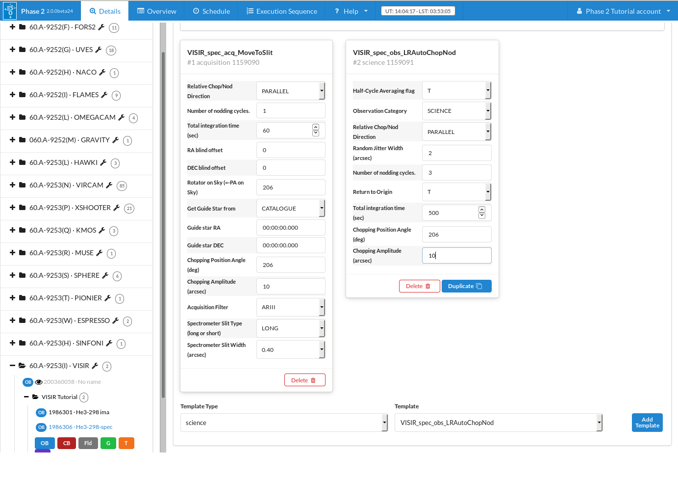
On Template Type, select now science. The existing VISIR science templates will appear. Select the template VISIR_spec_obs_LRAutoChopNod and click on Add. The template will be attached to the grid below next to the acquisition template selected and filled previously.

Several parameters have to be defined for this template. In the following we discuss each of them and justify a certain choice based on the properties of the target He3-298 and the scienctific goal of this spectroscopy OB. Since you want to chop and nod within the slit to use the full exposure time to integrate on-source, you select a parallel chop/nod direction, and the same chopping position angle and amplitude that you have selected in the acquisition template. You therefore enter:

• Relative Chop/Nod Direction: PARALLEL (Default value)
• Chopping Position Angle: 206
• Chopping Amplitude: 10

Several bad pixels or cosmics will produce an errornous response at some parts of the array. Therefore you want to avoid thetarget's signal falling permanently on a bad pixel and you chooseto jitter on the nod positions by setting:

• Random Jitter Box Width: 2

After using the exposure time calculator for VISIR in spectroscopy mode, you know that 500 seconds of total integration time is needed on He3-298 in order to reach the signal to noise ratio you want. To get a good sky subtraction we divide our 500 second integration in 3 nodding cycles. Thus,

• Total integration time: 500
• Number of nodding cycles: 3

If you followed all the instructions given so far, the View OB window should look like this now.

The only other thing that you should really do at this point is to check the execution time for this OB. Click on the Exec. Time tab at the top of the screen to re-calculate the execution time for your OB.

to the top

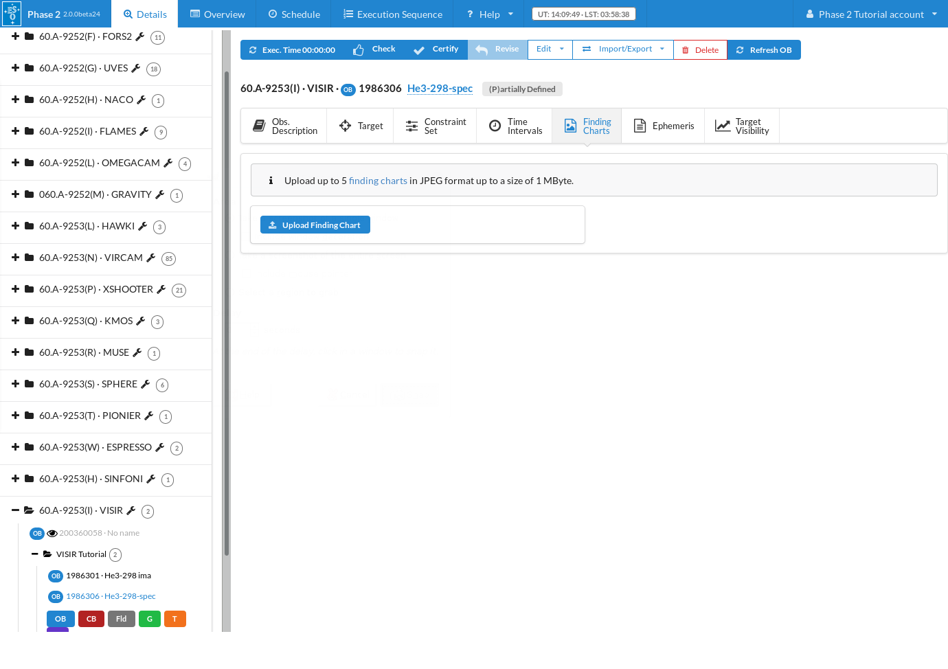
2.2.7:Attaching Finding Charts

The last thing to do, which finishes the preparation of a single OB, is to attach the respective Finding Chart(s) to the OB. The Finding Charts must be prepared as jpeg-files and must fulfillall general and VISIR-specific requirements for finding charts. You can use any tool of your choice to create the Finding Charts in jpeg-format. p2, however, does not contain such an option.

Let's assume you have prepared a jpeg-Finding Chart for this tutorial run [remember:run ID 60.A-9253(I)], which you called 60.A-9253I.he3-298.jpg, which is saved in a sub-directory of your home directory.

Now, in the p2 main window clickon the "Finding Charts" tab, and select the finding chart(s) which should be attached to the OB:

to the top

3: Finishing the preparation and submitting the OBs

With the completion of two OBs, we consider the examples developed in this tutorial to be finished. 

However, for a real run, you would also make sure to:

1. click the "Check" button (to the right of the Exec. Time button) for each OB.  This performs a number of consistency checks on the selected OB(s).
2. click on the Certify" button (to the right of the Check button).  Certify does the same as Check, but additionally (if the check was successful) marks the OB(s) as fully compliant and ready for ESO's review.  It also marks the OB(s) as read-only.
3. (optionally) select one or more certified OBs and click on the "Revise" button (to the right of the Certify button) to revoke the certified status and allow re-editing.  If this is done it steps 1 and 2 above should be re-done for the OB(s) in question.
4. complete the information in the README file
5. click on the "Notify ESO" button (to the right of the Revise button).  This will lock all certified OBs as well as the README, in preparation for ESO's Phase 2 review process.

As mentioned above, all users have access to the p2 demo facility.  And, unlike the situation that existed with p2's predessesor, P2PP, all OBs are created directly on the ESO database (there is no longer a "check-in" requirement).  Hence, all users can see what you leave behind.  Indeed, after a while, if not properly maintained, the p2 demo runs could and would get cluttered with all manner of OBs, containers, etc.  Thus, as a courtesy to the next user who follows this tutorial, we would like to ask you to finish these exercises by deleting the OBs, containers, etc. that you make.

Finally, please note that when looking at the tutorial run in the p2 demo facility you will see that both OBs are marked as (+) Accepted.  This is a state that these OBs have been set in (by ESO) solely to avoid them being inadvertently deleted from p2.

P2PP Documentation

• General documentation
• Tutorial for finding charts

VISIR P2PP Tutorial

• 0: Goal of the Run
• 1: Getting Started
• 2: Your First OB - Starting with P2PP
  • 2.1: Define an imaging OB with P2PP
    • 2.1.1: Filling in the Basic Information
    • 2.1.2: Defining the acquisition template
    • 2.1.3: Inserting Target Information
    • 2.1.4: Setting the Constraint Set
    • 2.1.5: Setting the time intervals
    • 2.1.6: Setting the Ralibration Requirements
    • 2.1.7: Defining the Observation Description
    • 2.1.8: Attaching Finding Charts
  • 2.2: Define a spectroscopic OB with P2PP
    • 2.2.1: Filling in the Basic Information
    • 2.2.2: Defining the acquisition template
    • 2.2.3: Inserting Target Information
    • 2.2.4: Setting the Constraint Set
    • 2.2.5: Setting the time intervals
    • 2.2.6: Setting the Ralibration Requirements
    • 2.2.7: Defining the Observation Description
    • 2.2.8: Attaching Finding Charts
  • 3:Finishing the preparation and submitting the OBs