
FLAMES p2 Tutorial
This tutorial provides step-by-step instructions on how to prepare a valid set of Observation Blocks (OBs) for observations to be executed with the Fibre Large Array Multi Element Spectrograph (FLAMES), the multi-fibre facility mounted on the platform Nasmyth A at the ESO VLT Unit Telescope #2 (Kueyen). The specifics of this tutorial pertain to the preparation of OBs for Period 105 onward. Please note that all the figures shown below can be clicked on to get higher resolution versions.
To follow this tutorial you should be familiar with p2 : the web-based tool for the preparation of Phase 2 materials. Please refer to the main p2 webpage (and the items in the menu bar on the left of that page) for a general overview of p2 and generic instructions on the preparation of Observing Blocks (OB). Screenshots for this tutorial were made using p2demo -- the demo p2 server, but should not differ in any significant way from one's experience in preparing your own OBs under your run on p2 -- the operational p2 server.
0: Goal of the Run
In this tutorial, inspired by the some of the remarkably successful programs carried out with FLAMES, we will prepare some example OBs for a study of chemical abundances in the globular cluster M67 using the combined mode GIRAFFE Medusa+UVES (we will use two of the high-res Medusa settings and one UVES setup). The purpose of this observational project is to observe a large number of stars in M67 in order to derive elemental abundances.
The observing strategy we want to implement is to observe a minimum of two hundred stars with Medusa fibres, and assign UVES fibres to the brightest objects in the field in order to achieve higher resolution and a larger spectral coverage. We will assume that we can cover all our target stars with two seperate fiber allocations centered on M67, meaning that we will use two different FPOSS setup files (INS file 1 and INS file 2). We will use Group containers to prioritise finishing the the two Mesdus settings for each FPOSS setup before starting the next FPOSS setup.
1: Getting Started
If you are reading this page, it is very likely that your program has been allocated time with FLAMES. Because of its 39 different wavelength/resolution setups (31 in high resolution and 8 in low resolution) and 3 different instrument modes (GIRAFFE, UVES, and the combined mode GIRAFFE+UVES), this tutorial will not be able to cover all the possible combinations: it is meant to give you a general overview and get you started with the Phase 2 preparation.
You can follow this tutorial without prior knowledge of FLAMES, but we recommend that you familiarize yourself with the documentation below before preparing your own OBs. This tutorial should then serve as a quick guide and reminder throughout the process, but the information contained in the documentation should always be your primary reference:
- The FLAMES User's Manual
- The FLAMES Template Reference Guide
- The FPOSS User's Manual
- The VLT Service Mode instructions.
- The p2 documentation referred to above.
More details on the instrument status and on FPOSS can be found respectively on the FLAMES Web pages and on the FPOSS tool Web page. Further useful information and tools for the OB preparation can be found on the User Support Services and Tools Web pages.
2: Making OBs
2.0: p2
For the sake of this tutorial, we will use the p2demo -- the p2 demonstration facility: https://www.eso.org/p2demo
This is a special facility that ESO has set up so that users who do not have their own p2 login data, or do not have a run on the given instrument, can still use p2 and prepare example OBs (for example, while writing a proposal to get the overheads right!). You cannot use it to prepare actual OBs intended to be executed (except if you export the OBs and then re-import them back into p2 -- i.e. the operational p2). When you want/need to prepare OBs for actual execution you will need use your ESO User Portal credentials for p2 (with http://www.eso.org/p2).
You can always tell at glance if you are in the demo or production environmentby the p2 menu bar across the top of the window which is orange in demo and blue in production.
After directing your browser to p2demo, the main p2 GUI will appear as follows:
Runs for a number of instruments appear in the lefthand column, since the p2 demo facility is used for all of them. Similarly, if you log into p2 (instead of p2demo) with your own ESO User Portal credentials, you will get the list of all the runs for which you are PI, or for which you have been declared as a Phase 2 delegate by the respective PI(s).
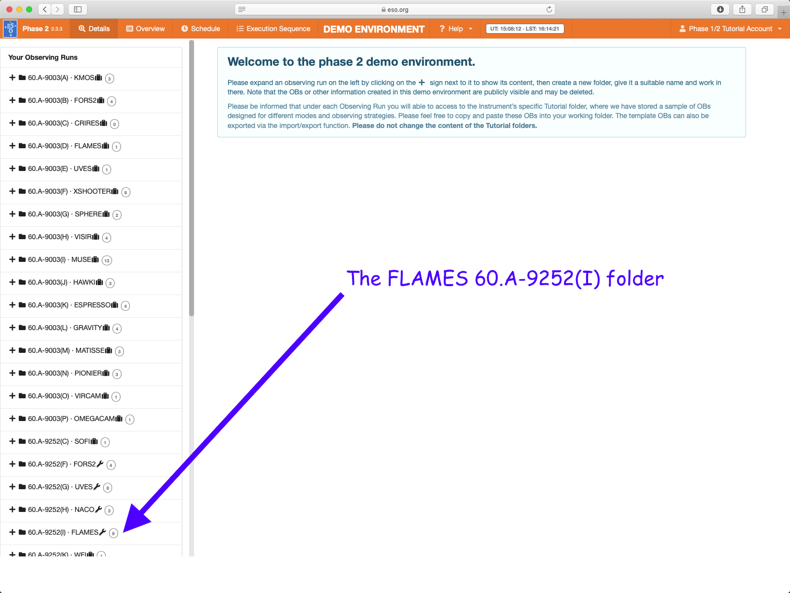
Open the folder corresponding to the UVES tutorial service mode run, 60.A-9252(I) (not the visitor mode 60.A-9004(D) run folder) by clicking on the + icon next to it. In this tutorial we assume that time was allocated in Service Mode. This is indicated by the small wrench icon that appears next to the "RunID - <instrument name>" label of the run (visitor mode runs have a suitcase icon in place of the spanner icon).
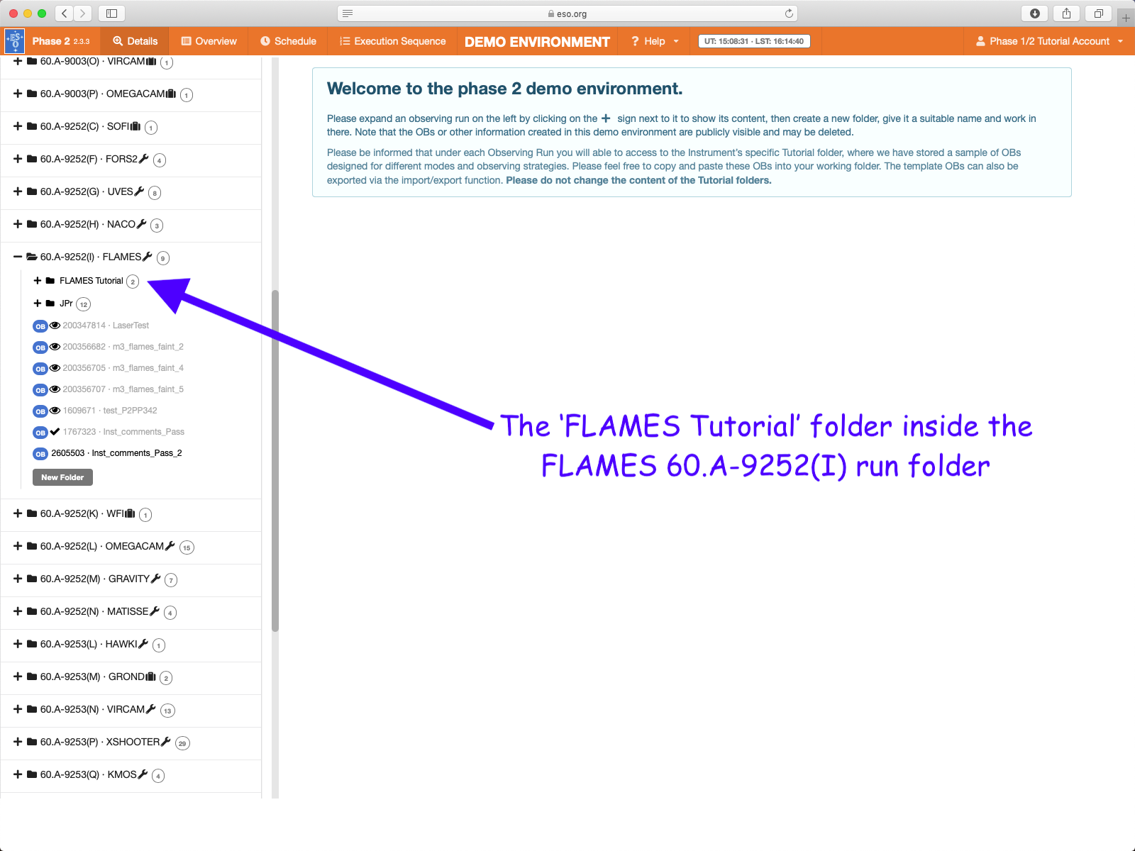
"Inside the run" you will see (at least) one folder, called "UVES Tutorial". That folder contains the final product of the tutorial you are now reading. You can refer to the contents of that folder at any time, perhaps to compare against your own work.
You can now start defining your observations. In the p2 demo you must first start by creating a folder, within which you will put your own content. Because the p2 demo is online and accessible to anyone you may see folders belonging to other people here, though after-the-fact cleanup is possible and infact encouraged.
First click on the "60.A-9252(I) · FLAMES" folder, then on the "New Folder" button at the end of the list of subfolders that already exist in the "60.A-9252(I) · FLAMES" folder. Your screen should look like this after you pressed the "New Folder" button:
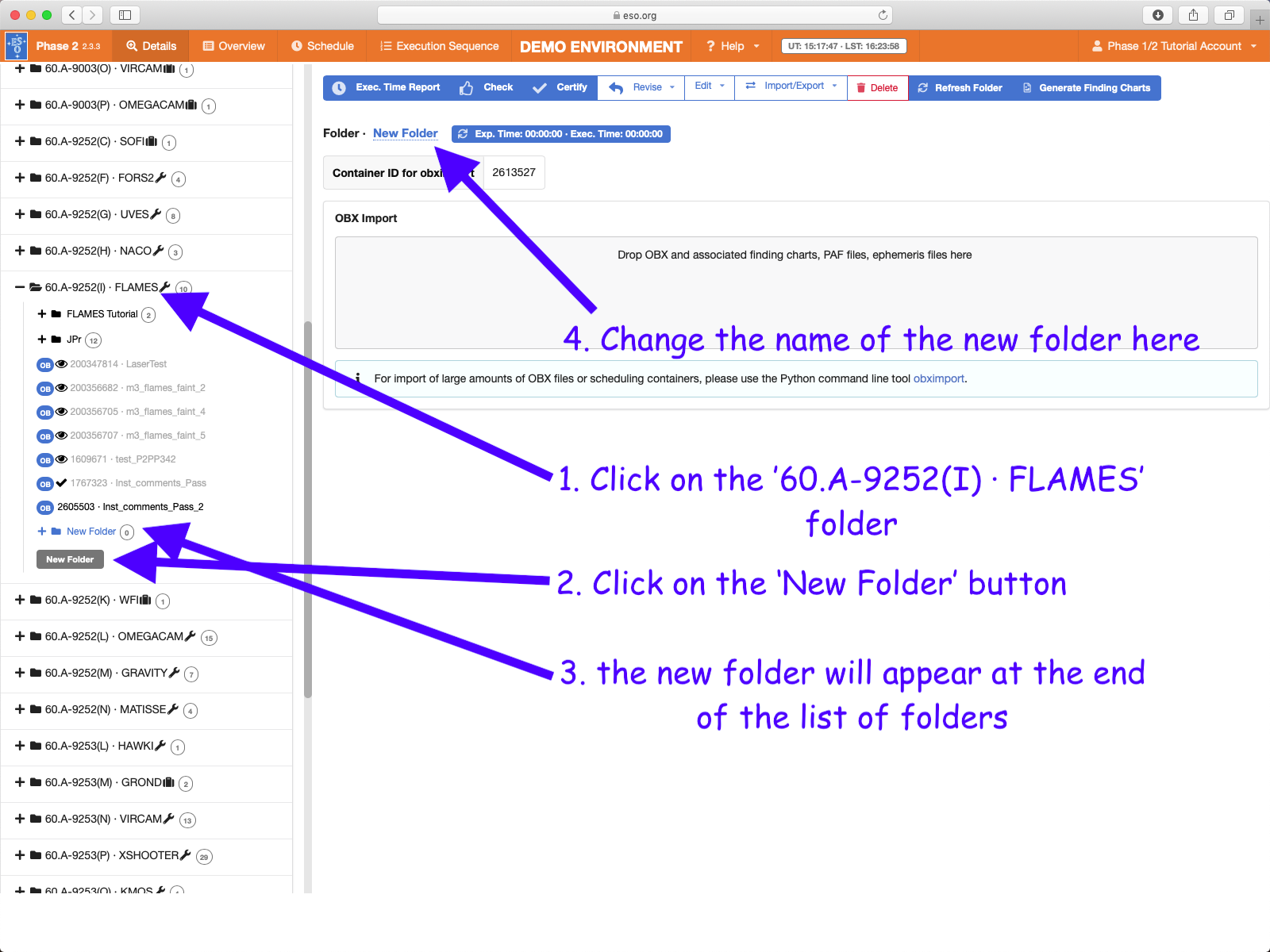
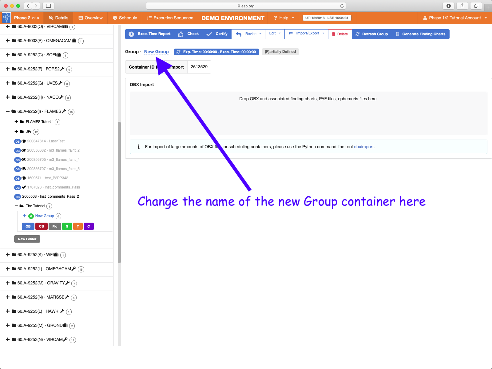
You can give the folder a new name by clicking on the blue 'New folder' text on the top, in this tutorial the name will be "The Tutorial", but you can set the name of your folder to be (almost) anything you like.
2.1: Creating OBs
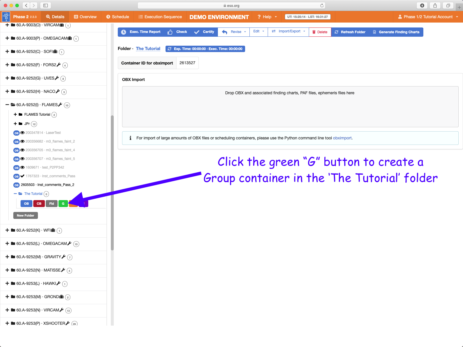
In order to start with the preparation of our OBs, since we want the two OBs with the two different MEDUSA settings to be executed for one FPOSS setup before starting the next FPOSS setting, we should define them inside a Group container. Open the new folder you created by clicking on the + icon next to it and then click on the green G icon to create a Group container.
The newly created Group container will automatically be selected and displayed in the main part of the window. Click on the blue name field near the top to rename the Group to "Setup 1":
To create the first OB, open the Group by clicking on the + icon next to it and then click on the blue OB button of the Group.
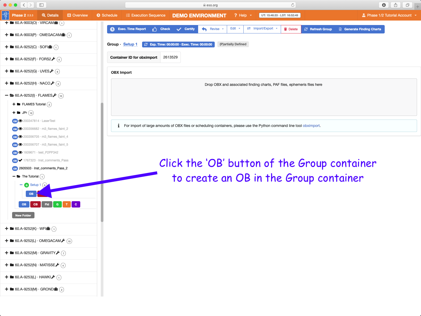
This creates the OB inside the Group container and it will be automatically selected and displayed in the main part of the window.
It is always a good idea to give meaningful names to OBs, so that you can browse through the list and easily recognize them. In our example, we will define OBs to take spectra of M67 with two MEDUSA settings for two FPOSS setups; for this reason we will call the first OB "M67 Setup 1 HR11" by renaming it as we did for the Group.
We could now also create the 2nd OB we will need, but it will be more efficient to complete the fisrt OB, duplicate it, and then just change the few things that need to be changed in order to observe the two different MEDUSA settings.
2.2: Setting the target information
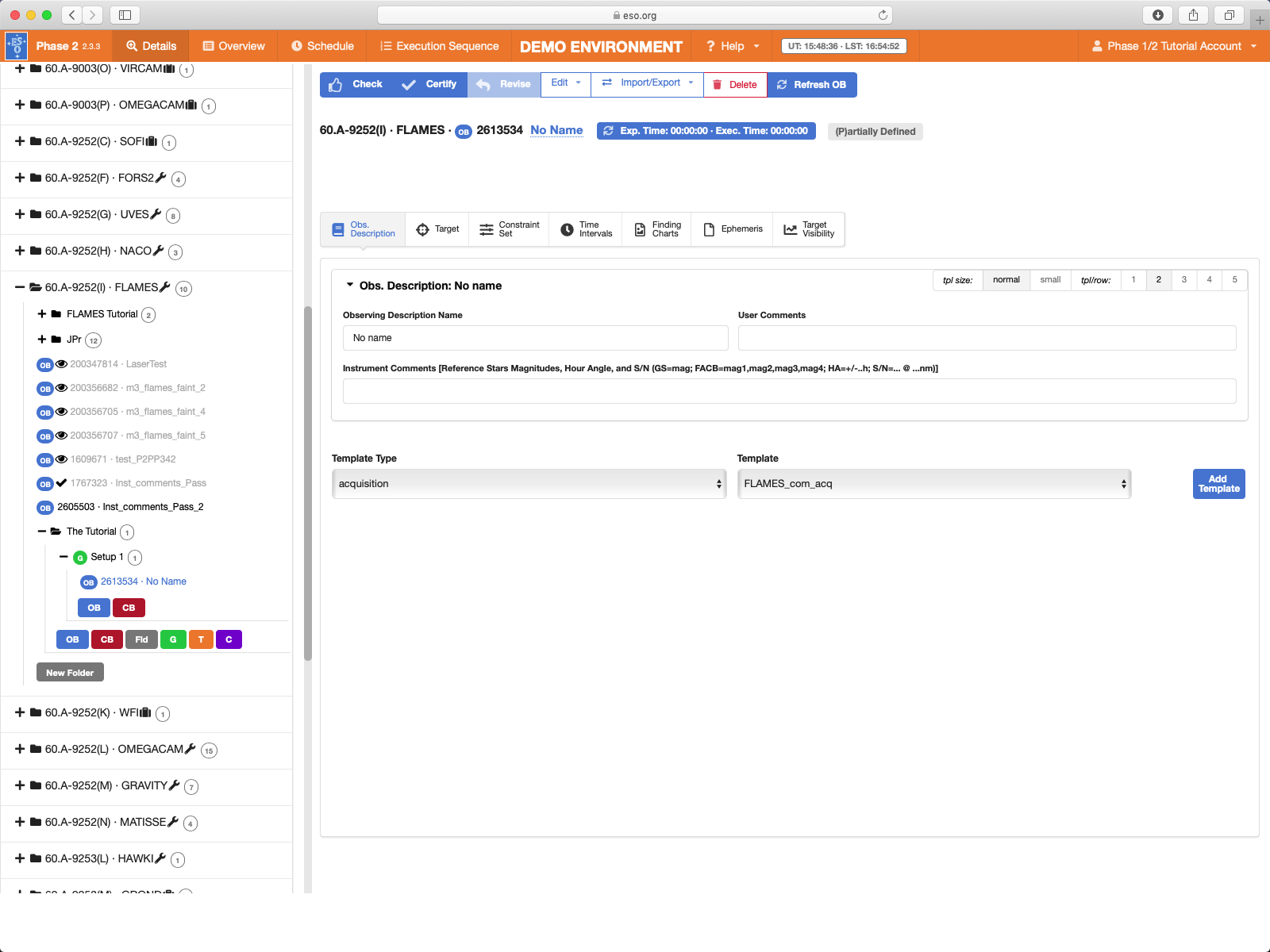
By default, the newly selected OB is displayed in the "Obs. Description" tab of the p2 tab bar (see above). You could enter the target information in the "Target" tab of the p2 tab bar near the top of the window, but for FLAMES the target information will be automatically updated from the FPOSS setup file once you attach it to the Acqusition template. You should not manually change the information in the Target tab, once it has been read from the FPOSS setup.
2.2.1: ObsPrep
The p2 built-in ObsPrep service only supports the ARGUS fast acquisition mode of FLAMES (Visitor Mode only). For all other observing modes FLAMES observation preparation is, as it has always been, done with the FPOSS.
We can thus proceed with the next steps...
2.3: Setting the constraint set
if your programme is in Visitor mode, you can ignore this section since you do not need to set the constraints for Visitor Mode OBs, but as stated in Section 1, we assume for the purposes of this tutorial that the program has been allocated time in Service Mode. You thus need to specify a constraint set for these tutorial OBs. You can do this by clicking on the Constraint Set tab and filling the fields accordingly.
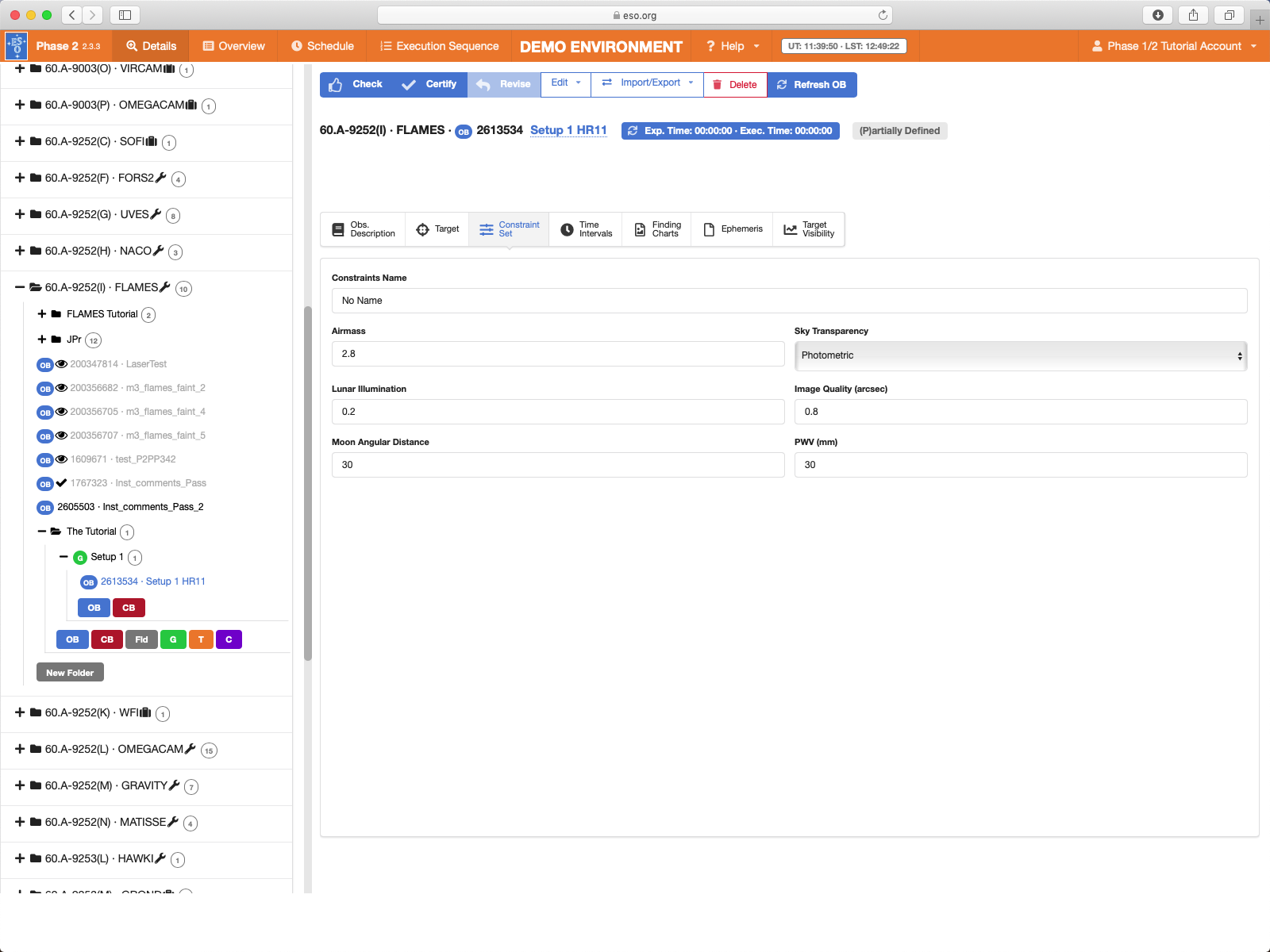
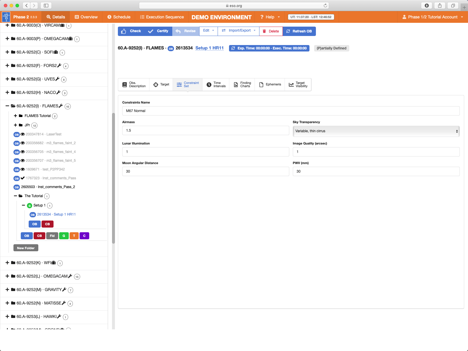
First, give a descriptive name to the constraint set about to be defined. In this case we choose "M67 normal" for the Name field.
Your actual constraints then need to be set to be compatible with what you specified in your Phase 1 proposal, and at the same time consistent with the scientific goals of you project and the awarded time. You should also take into account the OPC ranking of your run.
As a rule, you can not set stricter constraints than you specified in your proposal, but you can relax the constraints compared to your proposal (see the policy here). In general you should try to relax the constraints as much as possible (in order to maximise the chances for execution) whilst balancing the constraints and exposure times in order to still achieve the S/N you need to achieve your science goals.
Also consider that while we guarantee that IF your OBs are executed, they will be executed within 10% or better of your constraints, they could well be executed in significantly better conditions. So if you have very relaxed constraints, you may wish to consider nonetheless several short exposures, rather than one long exposure, in order to avoid the possibility of saturation in case the OB(s) is(are) executed in significantly better conditions than the specified constraints -- Alternatively, you can note in your README strategies that the observatory could employ to avoid saturation in such cases (e.g. "If executing in significantly better conditions than the constraints please decrease expsoure times to avoid saturation whilst maintaining the targeted S/N.")
As of P105, in your proposal you specified Turbulence Category, which for a non-AO instrument like FLAMES corresponds to a certain maximum Seeing, i.e. the image quality at the zenith in V-band (see here for a reminder). The table of Seeing vs Turbulence Category is reproduced below for your convenience:
| Turbulence Category | 10% | 20% | 30% | 50% | 70% | 85% | 100% |
| Seeing threshold | 0.5" | 0.6" | 0.7" | 0.8" | 1.0" | 1.3" | all |
In your OBs however you must specify Image Quality [IQ] at the wavelength of observation, the number you put in the Image Quality field of the OBs will not in general be the same as the Seeing value that directly corresponds to the Turbulence Category you specified in the proposal. In general for observations bluer than V-band you will need to specify a poorer IQ than the Phase 1 Seeing you specified, while for observations redder than V-band, you can often specify an IQ constraint better than the Phase 1 Seeing you specified. However you should also take into account the fact that the IQ at a given wavelength is degraded wrt to the IQ at the zenith.
You can use the FLAMES ETC to check what is the appropriate IQ constraint to specify for the phase 1 Turbulence Category/Seeing you specified. it is also often useful to experiment with the ETC with different combinations of airmass, moon illumination and distance, sky transparency and perhaps IQ to see how to best optimise the probability for successful execution of your OBs.
Alternatively you can also use the Check function of p2, which will tell you if you have specified an IQ that is not consistent with your Phase 1 Turbulence Category/Seeing, though you can't do this till the OB has at least a basic complete definition (see below).
So having experimented with the ETC for our present case we set the constraints as follows in order to achieve our science goals: Sky Transparency = "Variable, thin cirrus", Airmass = 1.5, Image Quality = 1, Lunar illumination = 1, Moon Angular Distance = 30 (degrees) and PWV 30mm.
2.4: Setting time intervals
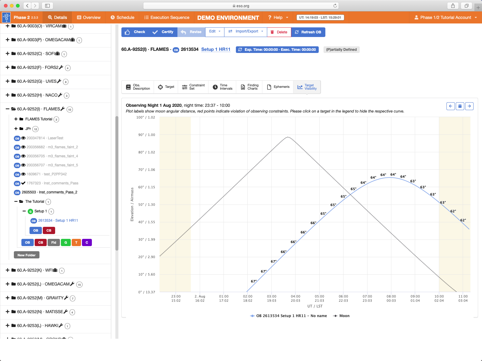
We will assume now that these of M67 observations have to be obtained during the period Aug 1 to Aug 25 2020, since you will have simultaneous observations at other wavelengths during that time interval. You can specify this by configuring time intervals in the Time Intervals tab.
p2 will present a representation of the allocation of nights at the telescope (unfortunately this functionality doesn't work in the p2demo environment).
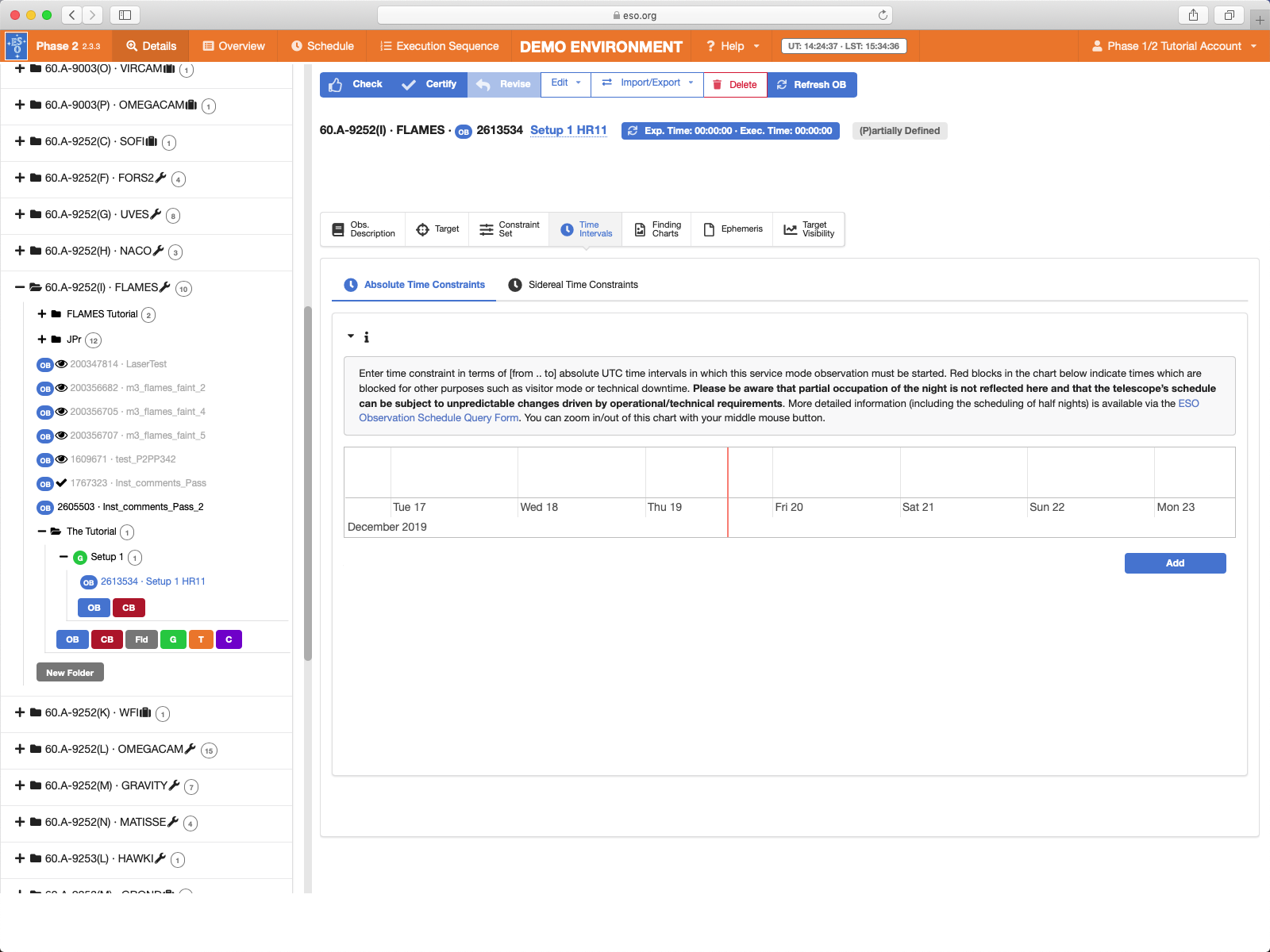
Red blocks represent nights that are not scheduled as full nights of Service Mode, so you should aim to have as many as possible absolute time intervals outside the red blocks. It is possible that serivce mode OBs can be executed during red blocks (e.g. because the particular night is a half-night of Service Mode) but you should not rely on this possibility just based on this view. More detailed information (including the scheduling of half nights) is available via the ESO Observation Schedule Query Form (see below). Please bear in mind though that the schedule does evolve during the period according to operational needs. Therefore include all possible absolute time intervals during the period, even if they fall entirely within red blocks.
To add an absolute time interval, just click the blue Add button below and to the right of the schedule. This will add a new "from" and "to" pair of fields, you can adjust the from and to dates and times by typing directly in the fields or by using the calendar (and following time) widgets to the right of each field.
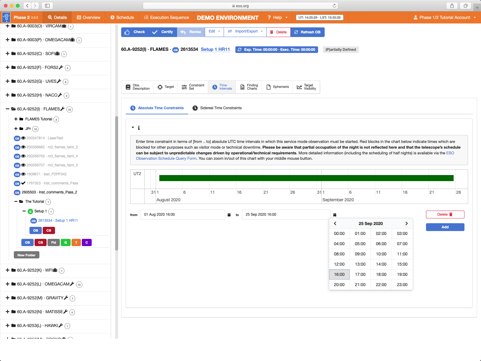
Once a valid interval has been entered it is displayed in the schedule view as a green block.
It is important to keep in mind that Absoute Time Intervals represent the intervals during which the OB can be started, not the intervals during which the OB must be started and finished.
For an interval like the one above this is not really an important distinction. But in certain situations it can be, for example imagine you wish to obtain spectra before, during and after a planetary transit. If you have (say) 4 hrs of OB(s) (with an approved waiver of course), and the transit lasts 3hrs, and you need at least 15mins of observations before and after the transit, then you will have just a 30min long window, starting 45+6mins before and ending 15+6mins (remember there is ~6mins of overhead from the start of an OB before any science spectra are taken, for most instuments, ~15 for FLAMES) the transit during which the OB must be started, and the Absolute Time Interval(s) must be set to these 30min intervals.
Each OB can have multiple time intervals (in general the more the better to improve the chances of execution). Just click the Add button to add additional interval(s). Each interval also has a delete button which allows you to remove intervals one by one.
The Target Visibility tool accessible via the Target Visibility tab is useful to check that your target is actually observable within your defined constraints during your defined time intervals.
Note that all time critical aspects (absolute time intervals and timelink containers) must also be explained in the section on "Time Critical Aspects" of the README (see the README tutorial here). Note, no need to list the specified Absolute Time Intervals, just explain why they are needed (e.g. for the planetary transit example above, 30min long Absolute Time Intervals specified in order to start the observations at least 15mins before the start of the 3hr long planetary transit and to finish at least 15mins after the end of the transit).
For more information on entering time constraints and how to use TimeLink containers to enter relative time constraints, see the generic p2 tutoirals here.
2.5: Defining the Observation
Click on the Obs. Description tab to return to the primary tab of the OB.
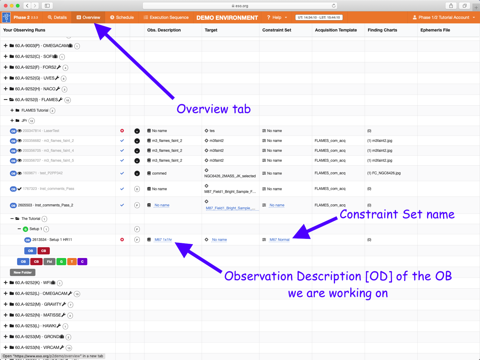
An OB is defined by a set of one or more templates that form the Observation Description, or OD for short. It may be useful in many cases to have an easy way of identifying an OD, like when having observations of a number of targets performed with identical instrument configurations and exposure times. The Observing Description Name field in the Obs. Description tab allows you to define name of the OD. The OD name appears in turn in one of the columns of the Overview tab, thus allowing the identification at a glance of all OBs having ODs with the same name.
In this example OB, the OD will consist of a single long exposure maximising exposure time whilst remaining within the 1hr OB limit. We can thus appropriately name it 'M67 1x1hr'. We enter this name in the Observing Description Name field, and we can now see this in the Overview tab.
Now back to defining the observations, click directly on the Details tab button next to the Overview tab button.
The first template that must be part of any science OB is the acquisition template, so let us define it first. In the Template Type pull-down menu, make sure that the acquisition entry is highlighted. Now we can select the appropriate acquisition template from the Template pull-down menu on the right.
For FLAMES there are only four different acquisition templates corresponding to the three instrument modes GIRAFFE-only, UVES-only, and the GIRAFFE+UVES combined mode plus one additional template, the FLAMES_giraf_acq_argfast for the ARGUS fast acquisition mode (no FPOSS setup file), which is only offered in Visitor Mode.
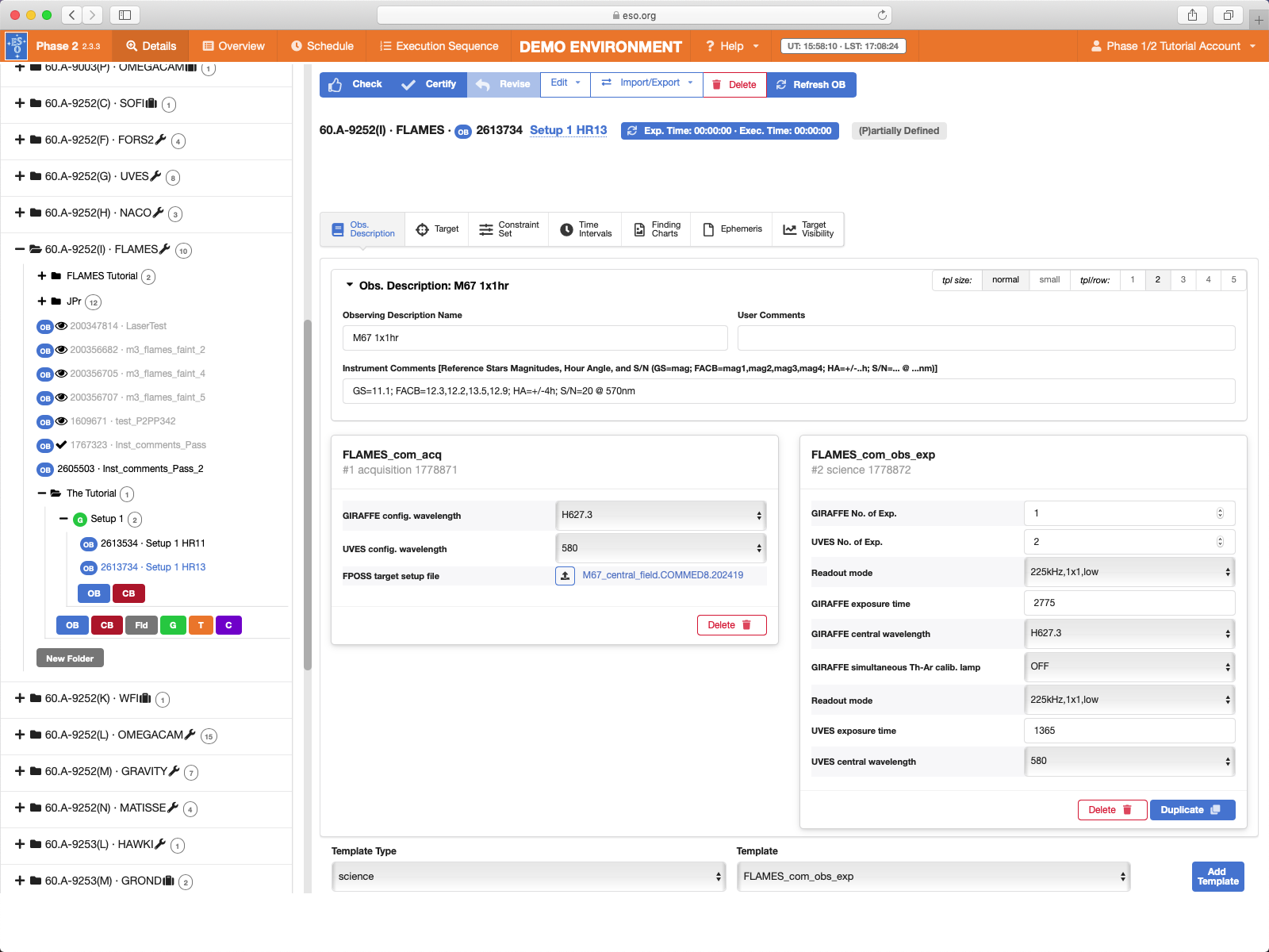
You must select the appropriate acqusition template corresponding to the FPOSS setup you will be using. Consistency is not checked by p2 immediately, but it will be verified when "Checking" and "Certiifying" the OB(s). The two FPOSS setups provided for this tutorial (INS file 1 and INS file 2) were created in the GIRAFFE+UVES combined mode, so you need to select the FLAMES_com_acq from the Template pull-down menu. Then click the blue Add Template button next to it.
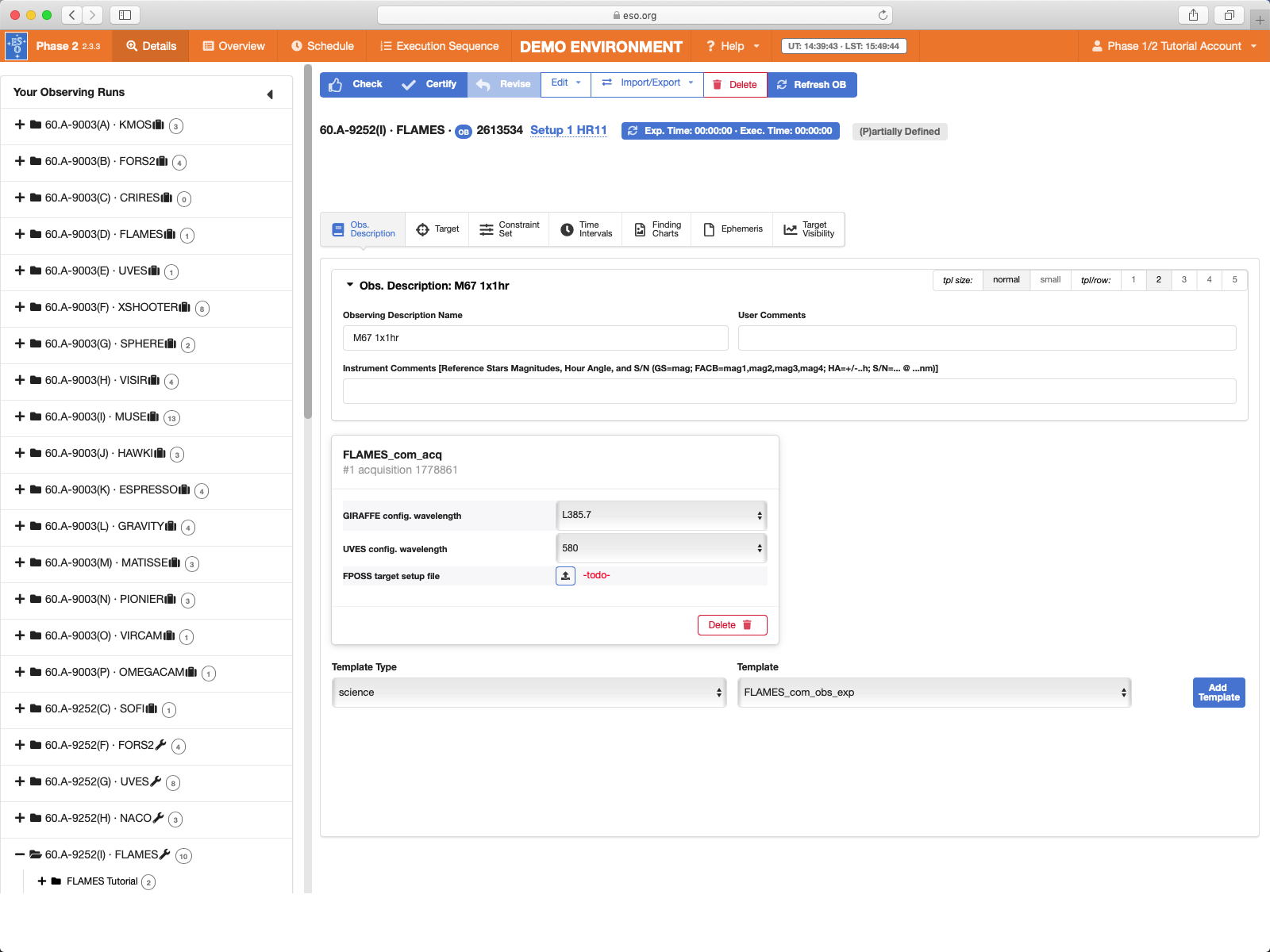
There are three fields that need to be edited: GIRAFFE config. wavelength, UVES config. wavelength, and FPOSS target setup file. For the configuration wavelengths we must select the wavelengths which our field(s) will be configured for (usually the wavelengths at which we will be observing) from the pull-down menus. Please note that the telescope will track on the GIRAFFE configuration wavelength. Depending on the target you are observing, the time at which the OB is executed and its total execution time, the difference between the MEDUSA and UVES configuration wavelengths (if any) may lead to increased fibre losses. This also applies to the IFU+UVES combined mode. In the FPOSS target setup file field we need to attach the previously prepared FPOSS target setup file (the *.ins file).
Our strategy is to use two GIRAFFE Medusa settings, HR #11 and #13, together with UVES Red_580. From the pull-down-menu corresponding to GIRAFFE config. wavelength let's start by selecting H572.8 (which corresponds to the central wavelength of setting HR#11 - please note that the default value of this field is always L385.7). As you may have noticed, there are some settings that appear to be double in the list and that can be distinguished only by a final A or B (or N, in case of HR#15). These settings have the same central wavelength, but are characterized by different spectral coverages and resolving powers. Please take a look at the table summarising all the high resolution settings of GIRAFFE. For the UVES part, we do not need to update the UVES config.wavelength because this value is defaulted to 580, which is exactly what we want.
Clicking on the upload file icon at the start of the FPOSS target setup file field, a dialog window pops up from which we can select the configuration file (the *.ins file) corresponding to this program. Note that the file is recognized even if the .ins extension is missing.
Once attached, the FPOSS target setup file field will be updated with the name of the selected file (without the .ins extension) and the Target tab in the OB window will be automatically updated with the Name, Right Ascension and Declination (see Figure). These values are read in directly from the .ins file, and they correspond respectively to the name of the target field and the coordinates of its center as specified in the header of the catalog file (the input file of our FPOSS session).

The acquisition template can then be considered complete.
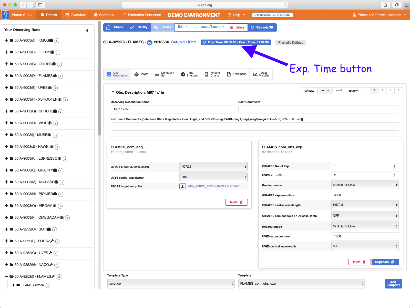
The selection of our science template is done in a similar way as for the acquisition. We just need to select science as our Template Type, then FLAMES_com_obs_exp from the Template pull-down menu. Then click the blue Add Template button next to it. As before, this will add the selected template to the OB. Again, the selected science template must be consistent with both the FPOSS setup and the acquisition template.
We can now edit the FLAMES_com_obs_exp template by specifying the number of exposures (in our case, 1 GIRAFFE and 2 UVES), the exposure times (3000 sec for GIRAFFE and 1500 sec for UVES), the central wavelength of our settings (572.8 nm and 580 nm respectively), and if we want to take simultaneous thorium-argon calibration data while integrating on our targets (ON or OFF - we turn it OFF, because for such a long exposure contamination from the the wavelength calibration lamp lines may affect the science spectra, as it is documented here).
Now click the blue Exp. Time button above the p2 tab bar (see below). The p2 server will calculate the OB execution time. For our desired exposure times of 3000 sec and 2x1500sec the total OB execution time is 01:04:30. Ooops. We thus need to reduce the exposure times. After some mental calulations and a few iterations we find that we can arrive at an executio time of exactly 01:00:00 with exposure times of 2775 and 1365, so we set the final execution times to those values.
This almost completes our first OB! We just need to fill out the Instrument Comments field (which is mandatory!), attach or generate a finding chart(s) (see below), and then "Check" the OB to make sure it conforms to the rules.
The recommended format for the comment is:
GS=mag; FACB=mag1,mag2,mag3,mag4; HA=+/-...h; S/N=... @ ...nm
So for this OB we enter:
GS=11.1; FACB=12.3,12.2,13.5,12.9; HA=+/-4h; S/N=20 @ 570nm
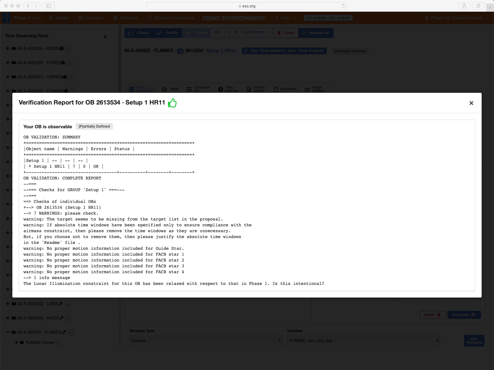
Now we can check that the OB conforms to the rules by clicking the Check button in the button bar across the top of the window, just under the orange bar. The check indicates 7 warnings, but no errors, so the OB is observable! We should probably check and if possible resolve all the warnings, but for the purposes of this tutorial, we will press on...
Click the x button in the top right corner of the window to close the Check report.
2.6: Attaching Finding Charts
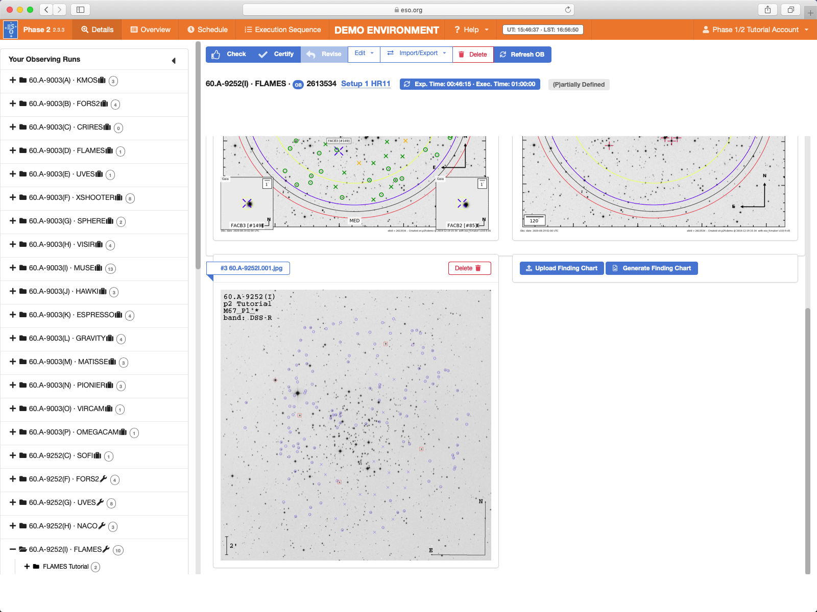
Finding charts must be attached directly to the OBs. Select the Finding Charts tab in the p2 tab bar.
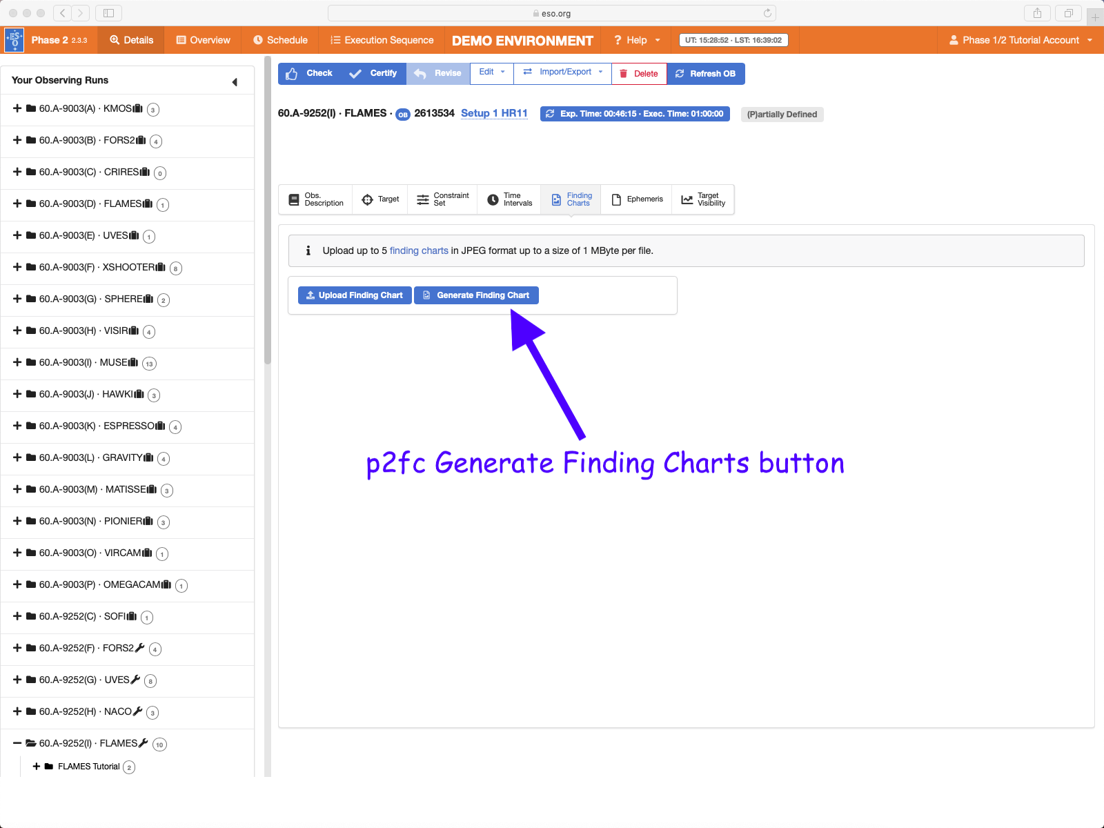
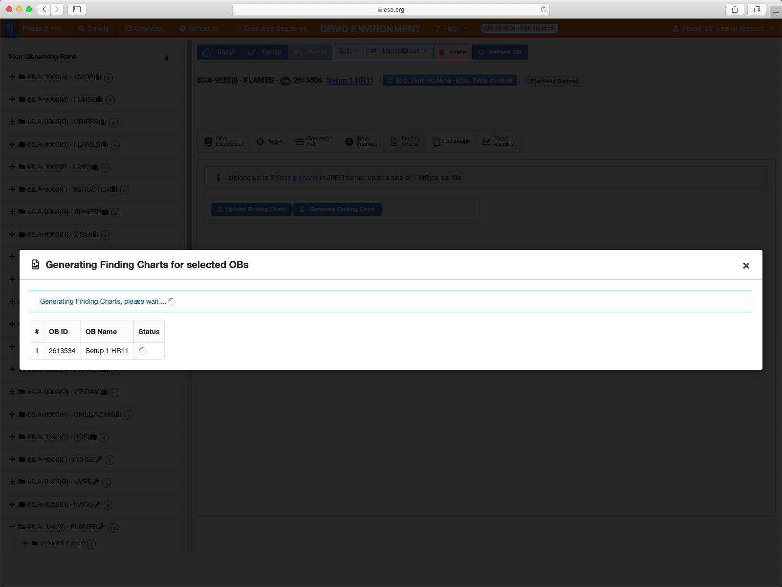
FLAMES is supported by the built in p2fc Finding Chart generating service. To attach standard defualt p2fc FCs to the OB, simply click the blue Generate Finding Charts button. When you click the button, a progress window will appear. A spinning indicator in the Status column indicates that the FC generation is in progress. When it is complete the spinning indicator will be replaced with "Done".
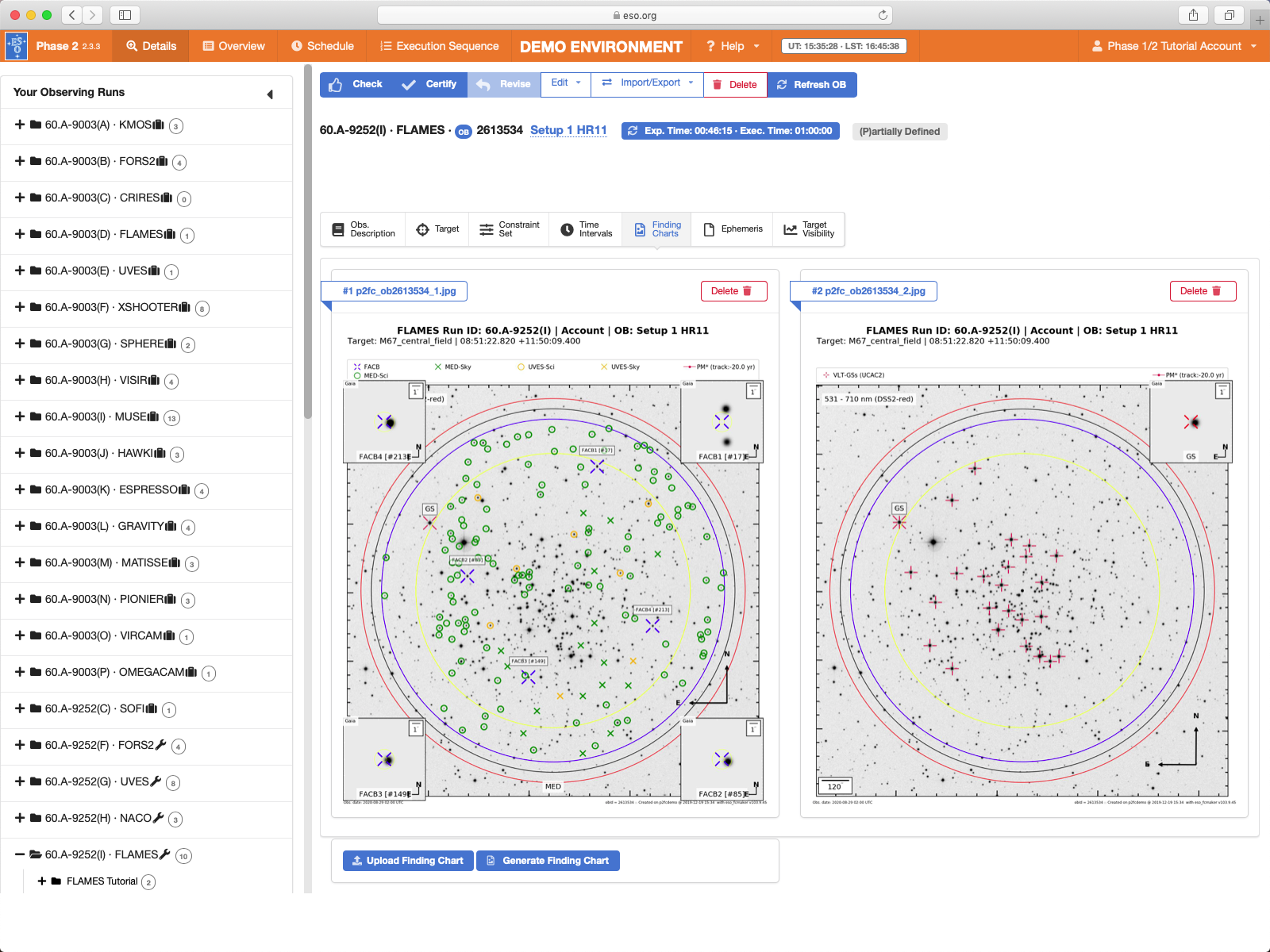
Once the FC is done, click the x in the top right corner of the FC progress window to close it and display the generated FCs.
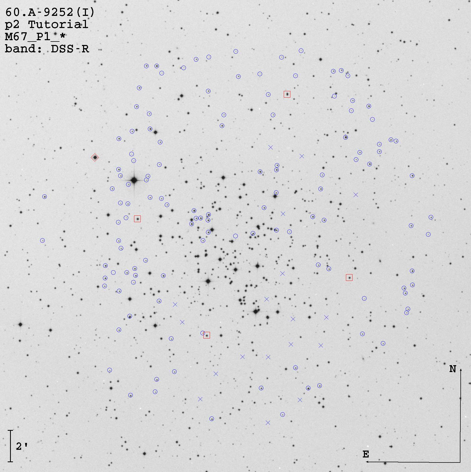
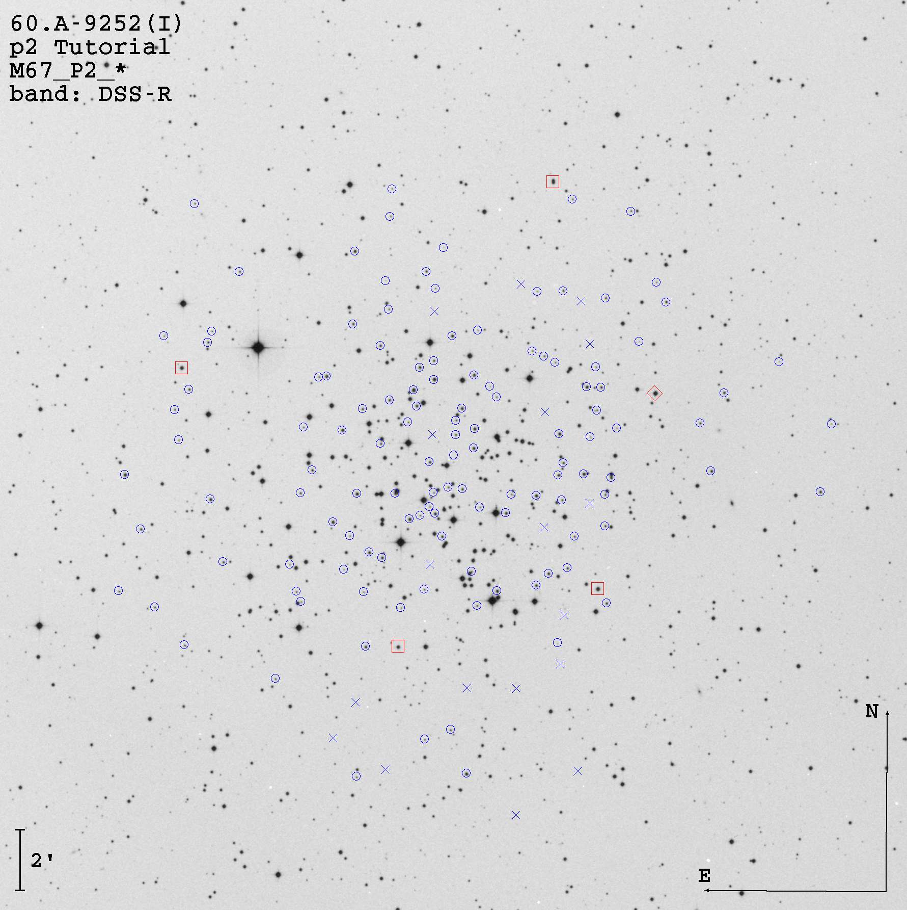
It is also possible to upload your own finding charts, see the guidelines here. Click the blue Upload Finding Charts button (to the left of the blue Generate Finding Charts button) and select the pre-prepared jpeg file(s) in the file chooser (you can download the two finding charts file used in this tutorial from INS file 1 FC and INS file 2 FC). Once successfully uploaded to the ESO database, they will also be displayed in the p2 window.
If you do attach your own FCs, it is generally a good idea to ALSo attach the p2fc ones too.
This completes your first OB!
2.7: Making more OBs
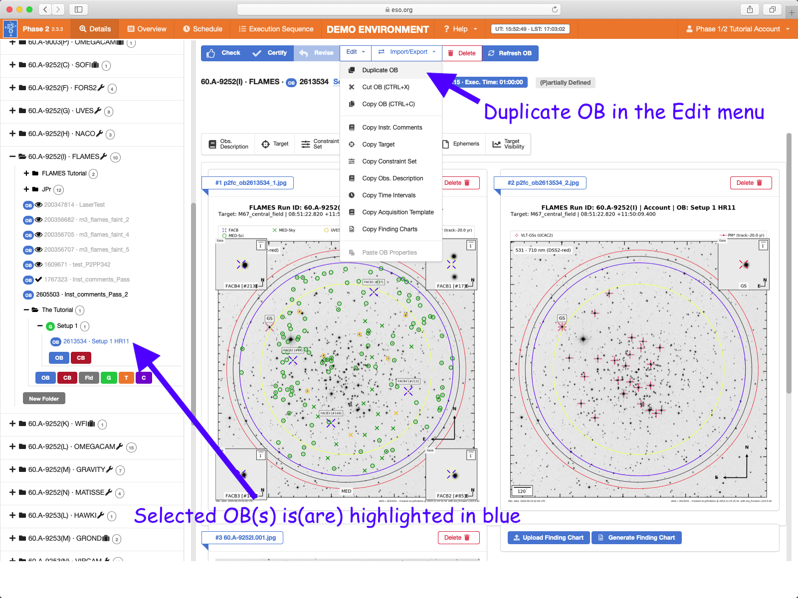
Since we also plan to observe the same field with the setting HR#13, we now need a 2nd OB. But it is almost identical to the first, so we can simply Duplicate the first one and then make the few necessary changes. Select Duplicate from the Edit pull-down menu in the OB tool bar.
Then in the new OB, change the OB name to "Setup 1 HR13", the GIRAFFE config. wavelength in the acquisition template and the GIRAFFE central wavelength in the science template to H627.3. And then re-generate the p2fc FCs.
To make a second Group container to observe the 2nd FPOSS setup, we just need to duplicate the entire current container, then change the Container and OB names and the FPOSS setup file in the acquisition templates, update the Instrument comments and re-generate and/or attach the correct Finding Charts of the two OBs.
This is left as an exercise for the tutorial follower, you can compare your duplicated and modified Group with the ones in the FLAMES tutorial folder.
3 The last steps: verification, README file and OBs submission
This tutorial is now completed.
As already mentioned, it has certainly not covered all the observing strategies you may have foreseen for your program, but it has shown how to prepare OBs for a representative case.
To complete a Phase 2 submission you would still need to:
- Complete the README
- Certify the OBs and containers
- Notify ESO
Please see the general tutorials here which cover these topics.