
CCD Tests
Test of electrical levels
Once the circuit was assembled, the levels of voltage in the KAF sensor socket were verified according this table:
If one level was wrong, it was adjusted using the potentiometers or changing the zenner diodes.
CCD sensor tests
The tests were carried out by Rodrigo Badinez. Prior install the sensor, it was taken an offset image without ccd, with the Pisco software. The average was about 460 counts, with a standard deviation of 10 units.
The next step was install the CCD sensor, and take a bias image (0 seconds exposition, 1x1 binning mode). The first obtained images were fully saturated, even in complete darkness. This leads to analyze the video signal with an oscilloscope, and we notice than the clamp circuitwas not working because the U7 amplifier was saturated. A resistance of10K ohms (named R100 in the schematics) inserted before the OpAmpsolve the problem.
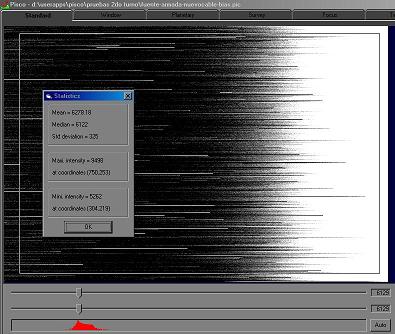
This way we took another bias image that wasn't saturated. The average of this image was about 6300 counts, with a standard deviation about 800 units.
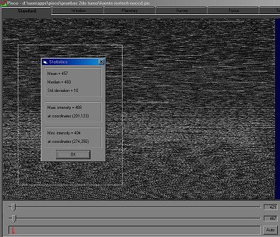
Offset Image without CCD (noisy)
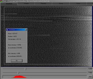
Bias Image, very noisy
First Light
For this test the camera was sealed and the test lens was installed. We try to get an image ofa coaxial cable connector, located approximately 1.2 meters away from the camera. The connector was illuminated only by a small torch. Hereafter isthe first light image.
The vertical lines are due the absence of the shutter, in the process of reading still photons are converted to electrons. Making the shutter effect "manually", and focusing more exactly, we got another image.
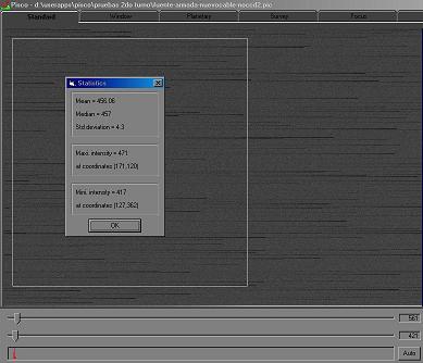
New power cable, Offset Image without CCD
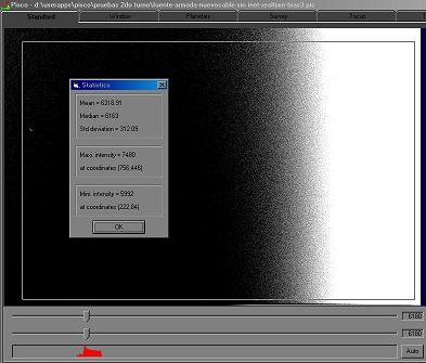
New power cable, Bias Image
On the offset image, the standard deviation was reduced from 10 to 4.3 units. On the bias, the standard deviation was reduced from 800 to 325 units.
As the noise is low, the horizontal lines stand out more. This lines doesn't appear to be related with the image, and are located randomly. That's suggested us that were reading errors, due to synchronism loss on the clocks generated by the computer.
To test this hypothesis, we close all the other running programs an process on the computer, take another image and check if the amount of line had diminish. And exactly that happened. Then we increase the priority of the PISCO process to real-time, and finally the horizontal lines disappears.
Bias Image with Real-time program priority
Finally I take some new pictures to see how much the image quality has improved.
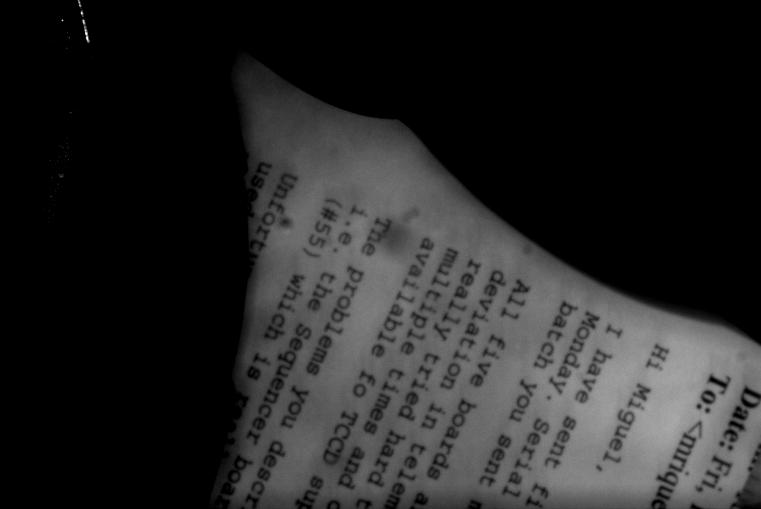
Picture of a letter, located about 1 meter from the camera (exp=3s).
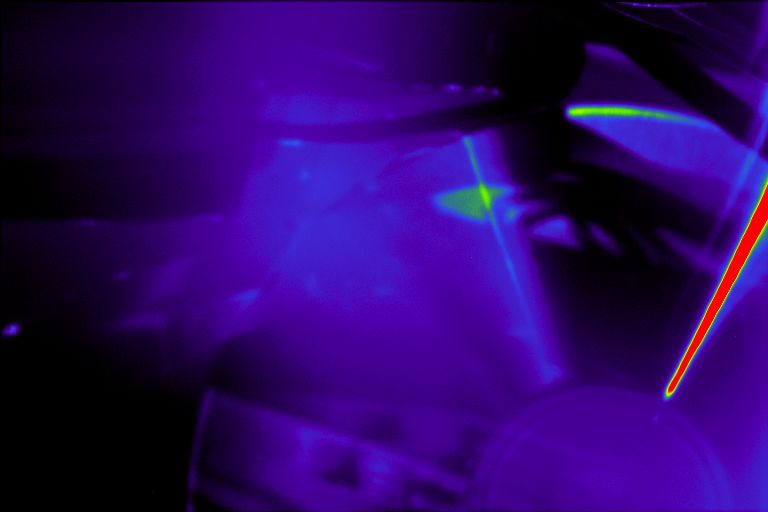
Picture of CD (exp=5s) with false color (rainbow) palette
Noise analysis with MATLAB
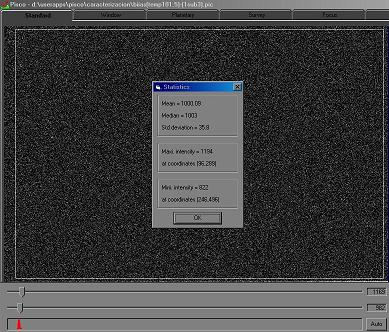
Subtraction of two bias images at the same temperature
In order to have an indicator of the amount of noise, using the PISCO software we calculate the subtraction of two bias image at the same temperature (same value of resistance on the PT-100).The following image was obtained (at 101.5 ohms): the mean value was 0.09counts, the median was 3 counts, and the standard deviation was 35.8 units.
As the image is the result of a subtraction of two, the readout noise is 35.8/sqrt(2)=25.3 ADU (Analog to Digital Units; in Audine 1 ADU equals a signal of 2 electrons). This value is a little higher than the expected, so Rodrigo Badinez made a frequency noise analysis in MATLAB. The method used was the following one, using the fftnoise2.m command.
- Read the FITS image and load it into the MATLAB Workplace as a matrix.
- Prompt the pixel clock, and the line frequency of the image.
- Calculate the one-dimentional Fourier transform to all the rows of the image.
- Generate a new image with the transformed rows, and export it to FITS format.
- Average all rows, and plot the result. Also plot the center line of the transformed image to compare it.
- Repeats the 3 previous steps, but now for the columns.
Hereafter are the plots of the transforms obtained for the bias image (temperature at 101.5 ohms). The frequency range is a theoretical reference, it's not verified.
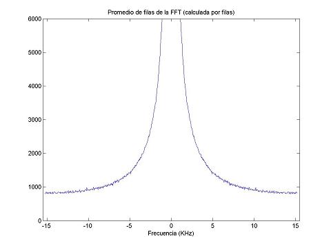
Average of rows FFT v/s frequency
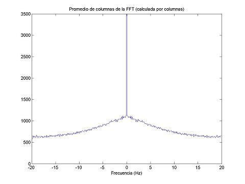
Average of columns FFT v/s frequency
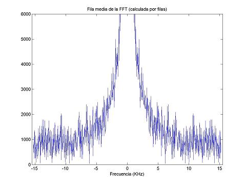
FFT of medium row v/s frequency
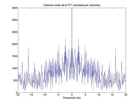
FFT of medium column v/s frequency
k on the average of FFTs (except of the central), therefore we conclude that the noise remaining is white noise. The most probable reason for this noise (on this camera) is the thermal Johnson-Nyquist noise from the resistances.
Lens used for the initial tests
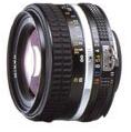
Nikkor lens
The lens used for the first tests, was the Nikon Nikkor 50mm/f-1.4, with a special adapter manufactured here in Paranal.
- Lens Type: Lens
- Maximum Aperture Range: F/1.4
- Minimum focal length: 45 millimeters
- Minimum Focal Range: 17.7 inches
- Focus Type: manual-focus
- Real Angle Of View: 46
- Mounting Type: Nikon F
- Weight: 8.1 Ounces
- Item Display Diameter: 2.6 inches